In Part 1, we saw that increasing the observation window changes the results for the occurrence of tails following heads. That raises the question: How does the micro (small observation window) relate to the macro (large observation window)? More specifically, what is the relationship between results from a small observation window (three flips) and those from a large observation window (100 flips)?
Many Collected Micro Events Are NOT The Same As A Macro Event
Blair Fix (Is Human Probability Intuition Actually ‘Biased’?) shows that the apparent bias in favor of tails following heads decreases as the observation window increases. Fix goes from an observation window of 3 flips to 5 flips, 10 flips, and ultimately 100 flips. When Fix repeats 3-flip sequences many times and accumulates the results, these accumulations are unconnected to the results for any other n-flip sequence(s). The accumulated micro-events of one type (type = number of flips) are unrelated directly to any macro-event constituted by many successive coin flips of other types.
Let’s recall two graphics from Part 1 that show the results of simulated iterated coin flips using random number generation.
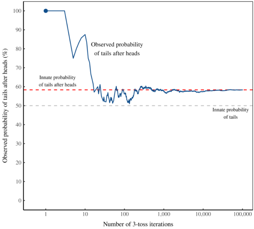
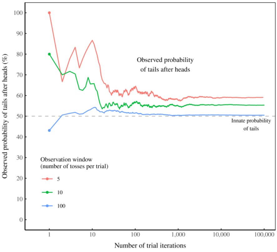
The graphs above show the “bias” favoring tails following heads decreases from 58% for an observation window of 3 flips to almost no “bias” with 100 flips.
When the observation window is unlimited, Fix shows a sample result of successive coin flips:
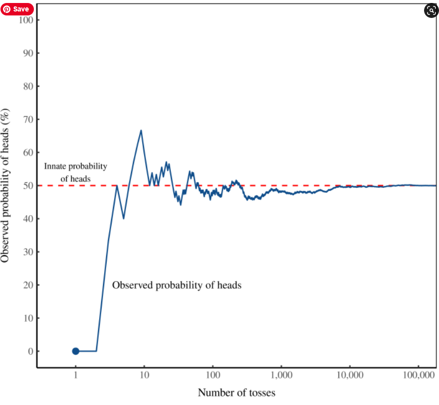
Figure 1: In search of ‘innate’ probability. I’ve plotted here the results of a simulated coin toss. The blue line shows the ‘observed’ probability of heads after the respective number of tosses. The red line shows the ‘innate’ probability of heads (50%), which is embedded in the simulation code but inaccessible to observers.
Fix shows that there are transitions from an accumulation of micro-results through progressively larger (‘less-micro’) events to a macro-event.
Why Do Collections Of Micro Events Differ From Related Macro Events?
One significant reason arises from the fact that macro-events contain not just component micro-events. They also contain interactions between the micro-components.
Let’s illustrate what we mean. The micro-events we have here are 3-flip sequences that have 8 equally probable sequences:
- HHH
- HHT
- HTH
- HTT
- THH
- THT
- TTH
- TTT
When we collect a number of these sequences, that collection differs from an equal number of individual coin flips. Could this be because the collection of sequences has no provision for connecting the individual sequences into a continuous flow?
Connections Of Sequences Change The Counts of Tails Following Heads
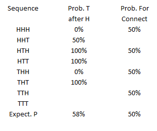
There are 4 sequences above ending with heads. The next flip following each of those heads has an equal probability of producing heads or tails. Let’s add the connections between micro-events to the micro-event results.
First, from Part 1:
Including the connections following each micro-probability distribution creates the following table:
Simply recognizing the T follows H probability for the connection to the next sequence might lower the “bias” by as much as half to 54%. This applies to each sequence except the last in the accumulation. As the number of sequences accumulated increases, the effect of the last sequence diminishes. The last sequence connection effect approaches a negligible amount for a large number of sequences, ie, much larger than 1,000. And, of course, the connection effect does not explain the difference between the innate heads/tails probability of 50/50 that we are observing.
Note: This example is purely illustrative. As will be shown in future parts of this series, the probability table we have used so far is not a complete description of what is experienced in reality. Reality is represented by the simulation graphics produced by Fix (shown above). The combinations of sequences involved are orders of magnitude greater than the one probability table we have considered thus far.
Counting Heads Instead of Sequences
In the section above, we determined the probability of a tail following a head in a sequence of three coin flips was 58%, different from the innate probability of 50% for a head or tail on any individual coin flip. The reason for the discrepancy is illustrated in the table below, which compares counting qualified sequences (repeated from above) with counting qualified heads.
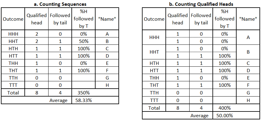
Once the counting is changed to counting heads rather than sequences containing heads, the observed probability is the expected 50%.
Increasing the Size of Sequences
In a preceding section, it was suggested that going from a sequence of three coin flips to four might lower the apparent “bias” favoring tails following heads. Here is a look at that.
Sequences flipping a coin four times
The table below compares results for the probability of a tail following a head in a sequence of four coin flips (a) and when counting qualified heads in that sequence (b).


The results above show that the “connecting Hs” do not explain the deviation of probability results from the single flip 50%. The probability in the sequence has risen to 59.5% from 58% in the three flip sequence. However, the probability of a tail following a head remains at 50% when based on counting qualified heads.
Sequences flipping a coin five times
Below, we repeat the previous calculations for a sequence of five flips. We do not show the calculations for qualified heads, which still produce a 50% probability.

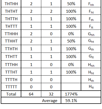
Now, the probability of a T following an H has dropped from 59.5% for a sequence of four flips to 59.1% for five flips.
Larger sequences
The graph below contains the data above plus the data above plus the simulations run by Fix for larger sequences.
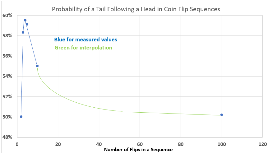
Even for a sequence of 100 flips, the probability still exceeds the single flip value of 50%. Indeed, we can expect that for any larger number of flips, the probability will approach 50% but never exactly reach it, short of an infinite number of flips.
What Sample Size is Needed to Reach the Probability Table Value?
The simulations run by Fix give data that addresses the question of how increasing sample size affects the accuracy of determining the probability bias of various coin-flipping sequences. The point at which the probability of a tail following a head stabilizes at the probability array (table) value is shown in the following table and the subsequent graph:
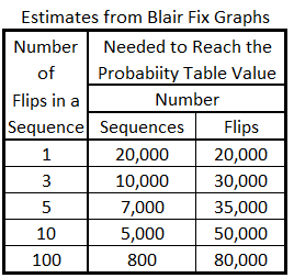

The bias for the probability of tails following heads may decrease as sequence sizes increase, but the number of flips needed to approach the probability array value and remain stable increases. Conversely, the number of sequences needed declines as the number of flips in a sequence increases.
Conclusion
The experiments shown above lead to several conclusions. Important among these:
- Flipping a coin a few times will not often produce results closely related to the innate probability indicated by probability calculations.
- Sample definition is important. Samples must be representative of the factor being measured. Measuring coin-flipping sequences can yield unexpected results when different sequences contain different populations of the parameter tested.
- When characterizing the performance of a simple process, a very large number of processes must be executed to be sure of approaching a statistically representative result.
We are now left with the questions:
- Why do the probabilities of a tail following a head vary with the number of flips in a sequence?
- Why are so many sequences necessary to ensure the probability of a single set of sequences?
Next – Part 3: Possibilities vs. Realities
Caption graphic: Photo by Mario Heller on Unsplash.
