M2 Money Supply and CPI Inflation. Part 2

The full data sets for the 64 years from 1959 to 2022 show no discernable association patterns (correlations) for M2 money supply growth and consumer inflation changes.¹ This post continues that analysis by looking specifically at the various regimes of inflation change during the 64-year timeline.

From an image by Qubes Pictures from Pixabay

Introduction

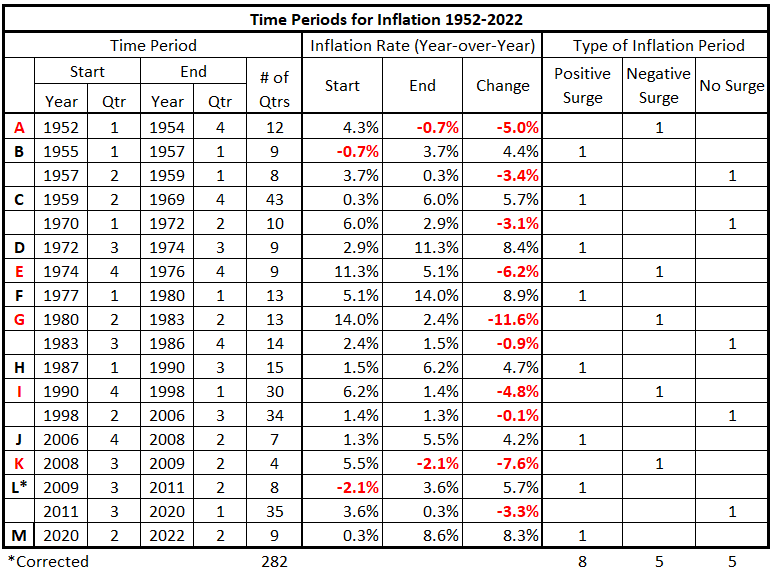
The 71 years from 1952 to 2022 are divided into three types of inflationary behavior:¹

Significant inflation increases;
Significant inflation decreases;
No significant inflation changes.

An inflation change is significant if it is ≥4.0% with no intervening countertrend change >1.5%.

Previously, we defined the partitioning of inflation into the pattern in Table 1.

Table 1. Timeline of Inflation Data 1952-2022 (Previously Table 4*.²)

We will examine each category of inflation behavior separately. In this piece, we analyze the significantly positive periods of inflation (positive inflation surges).

Data

The data is from Tables 5-17, prepared previously.¹

There are 13 quarterly timeline alignments:

M2 Money Supply and CPI Inflation quarters are coincident.
M2 Money Supply leads and lags CPI Inflation by one quarter (±3 months)
M2 Money Supply leads and lags CPI Inflation by two quarters (±6 months)
M2 Money Supply leads and lags CPI Inflation by three quarters (±9 months)
M2 Money Supply leads and lags CPI Inflation by four quarters (±12 months)
M2 Money Supply leads and lags CPI Inflation by six quarters (±18 months)
M2 Money Supply leads and lags CPI Inflation by eight quarters (±24 months)

Analysis

2Q 1959 – 4Q 1969

By our definition, the period from 1959 to 1969 constitutes a period of inflation growth—inflation growing by 4% or more without a pullback greater than 1.5%. However, the decade can be divided into slower inflation growth (1959-1964) and more rapid growth (1965-1969). Therefore, we analyzed the association between M2 Money Supply and inflation in these periods.

2Q 1959 – 4Q1964

Figure 1. M2 Money Supply and Inflation 1Q 1959 – 4Q 1964

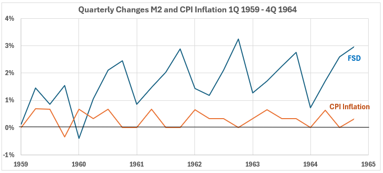
The quarterly change trend in the M2 money supply increased for much of this period, while the quarterly changes in inflation showed a flat trend. The magnitudes of the M2 changes were consistently larger than those of CPI, and the volatility was greater.

Figure 2. Quarterly Changes in M2 Money Supply (x) vs. CPI Inflation (y) 1Q 1959 – 4Q 1964

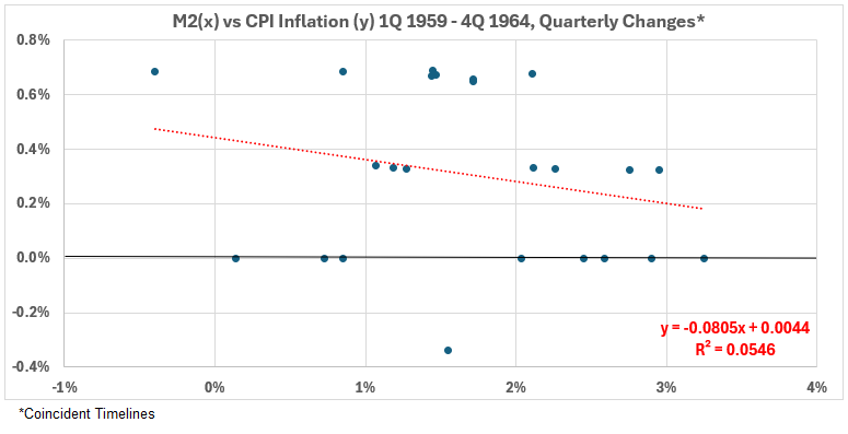
This scatter diagram shows a very weak negative association for the coincident timeline data. R = –23%, R² = 4.3%.

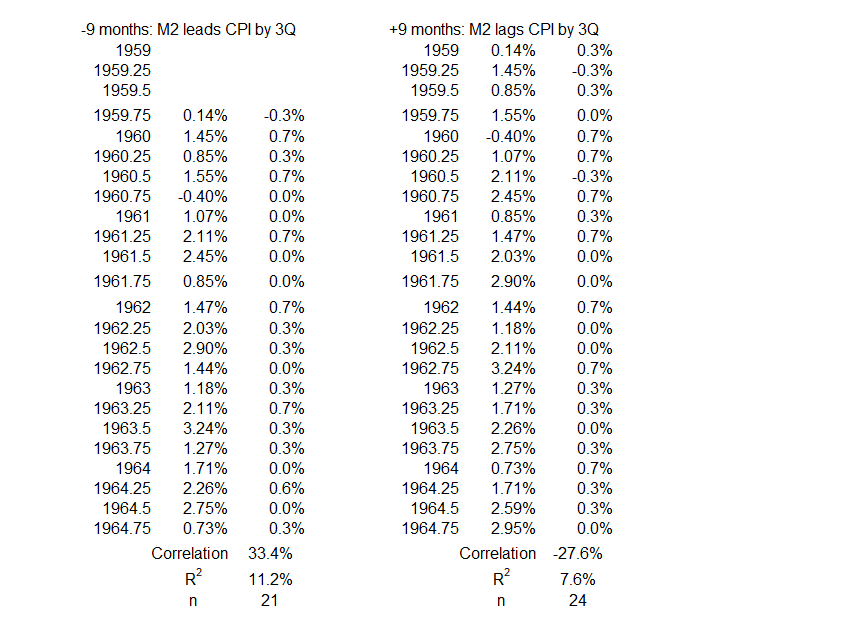
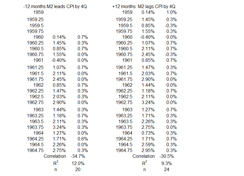
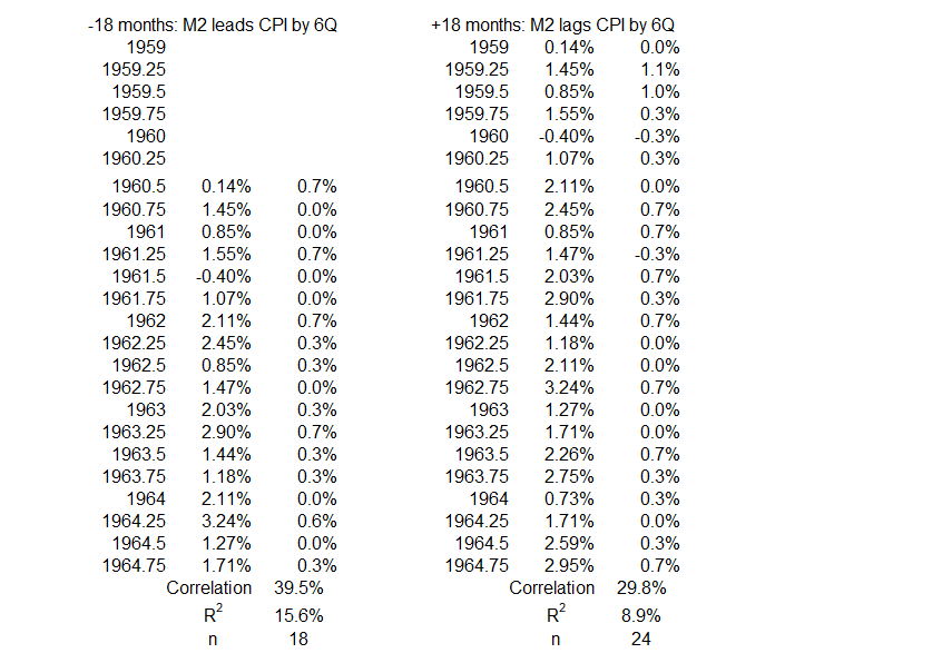
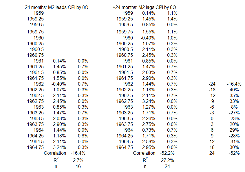
Figure 3. Correlation Between M2 Money Supply and CPI Inflation 1Q 1959 – 4Q 1964

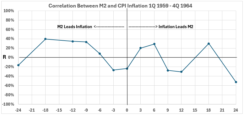
The two variables had a weak association during this period for M2 changes coming 9 to 18 months before CPI changes (left side of Figure 3). The R² values are 11%, 12%, and 16%. This means that the maximum possible effect of M2 changes on inflation was 16%. Other factors must have accounted for 84% or more of CPI inflation during this period.

The right side of Figure 3 indicates that CPI inflation changes might have accounted for small changes in the M2 money supply in both the same and opposite directions (R² < 10%, except for 24 months). That seems an unlikely situation, so, for now, we will consider these small associations coincidental.

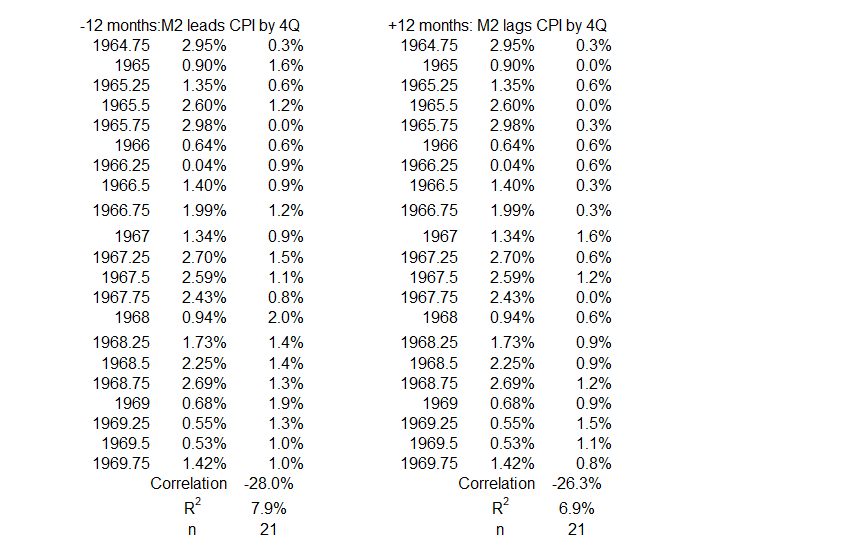
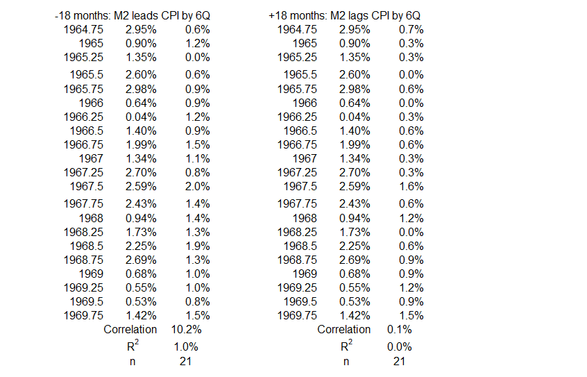
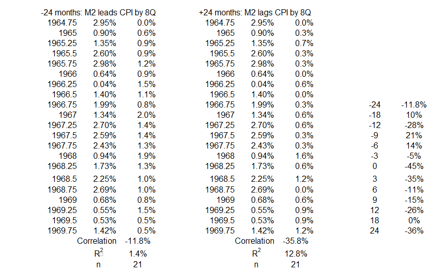
1Q 1965 – 4Q 1969

Figure 4. M2 Money Supply Growth and Inflation 1Q 1965 – 4Q 1969

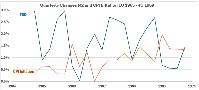
In Figure 4, the trend is negative for M2 changes but with great volatility. The trend for CPI changes is positive. Many of the M2 changes are larger than any CPI change.

Figure 5. Quarterly Changes in M2 Money Supply (x) vs. CPI Inflation (y) 1Q 1965 – 4Q 1969

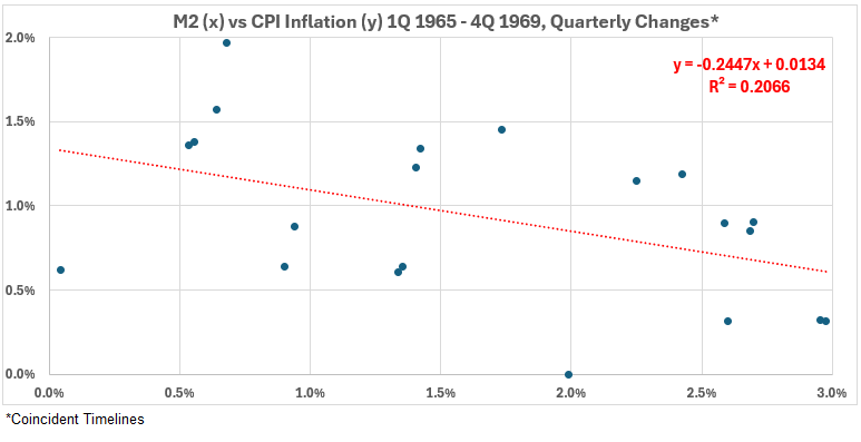
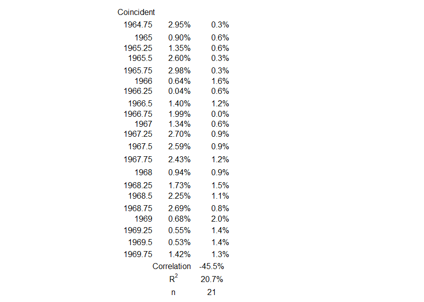
The coincident timeline data has a weak negative association, R = –45%, R² = 21%.

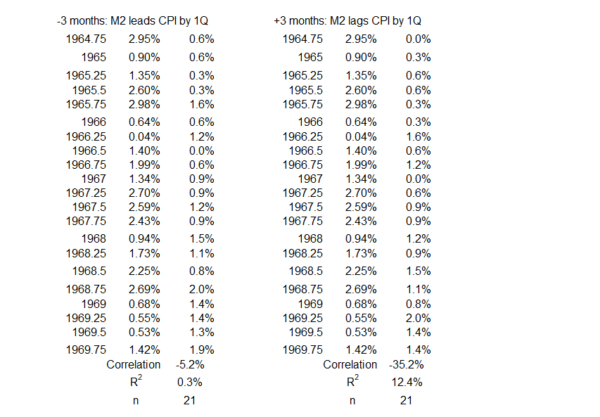
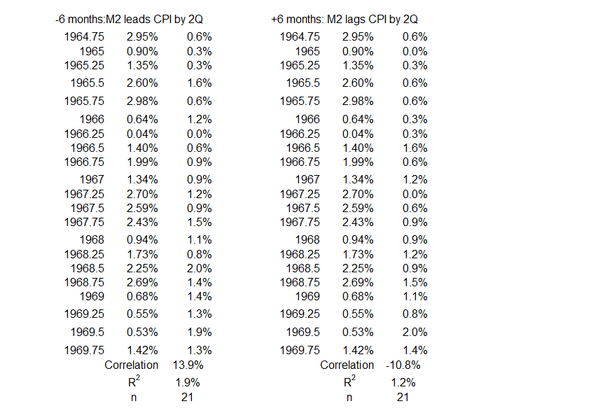
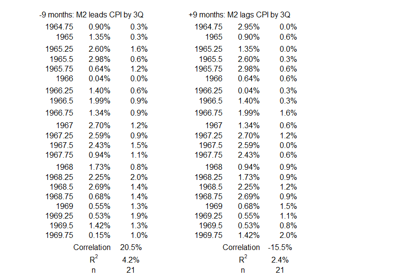
Figure 6. Correlation Between M2 Money Supply and CPI Inflation 1Q 1965 – 4Q 1969

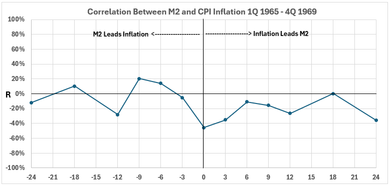
There were weak or negligible associations between the two variables during this period. Because no meaningful lead/lag relationships exist, it is unlikely that there were any cause-and-effect relationships between M2 money supply changes and inflation during this period.

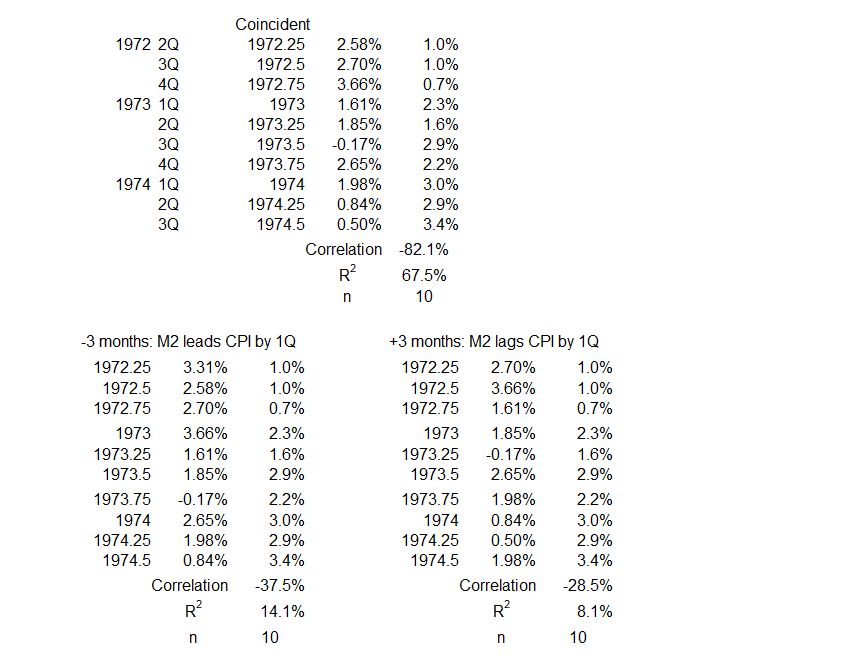
3Q 1972 – 3Q 1974

Figure 7. M2 Money Supply and Inflation 2Q 1972 – 3Q 1974

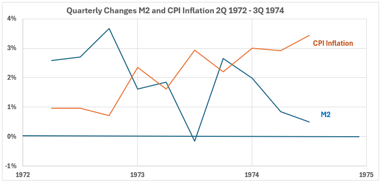
The changes in the two variables had opposite trends during this period, with M2 changes decreasing (albeit with large volatility) and CPI changes increasing.

Figure 8. Quarterly Changes in M2 Money Supply (x) vs. CPI Inflation (y) 2Q 1972 – 3Q 1974

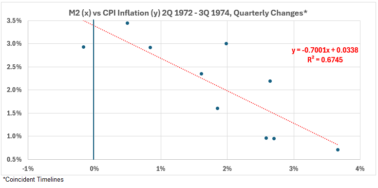
The coincident timelines data shows a strong negative association (R = –82% and R² = 67%).

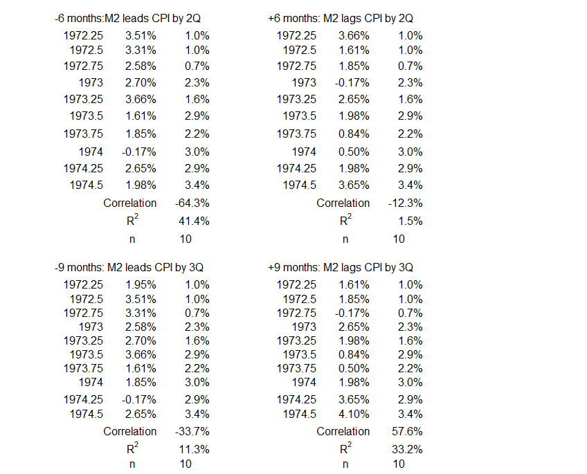
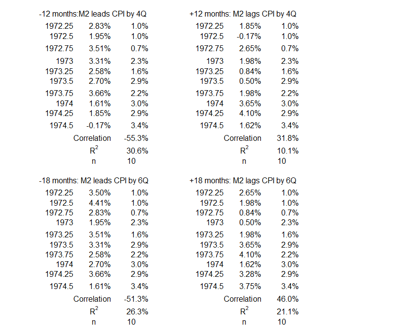
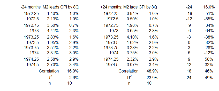
Figure 9. Correlation Between M2 Money Supply and CPI Inflation 2Q 1972 – 3Q 1974

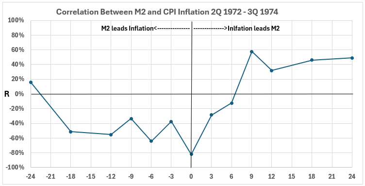
The left side of Figure 9 shows that there is no possibility that increasing M2 changes could have caused increasing CPI changes during this period. The exception is when M2 leads CPI by two years. In that case, R = 16% and R² = 3%. Thus, 97% or more of the increasing CPI must have come from sources other than M2.

The right side of Figure 9 indicates that CPI increases are associated with M2 increases 9-24 months later. The correlations are 58%>R>32%, corresponding to 34%> R²>10%. How much of this is possible cause and effect depends on obtaining additional information.

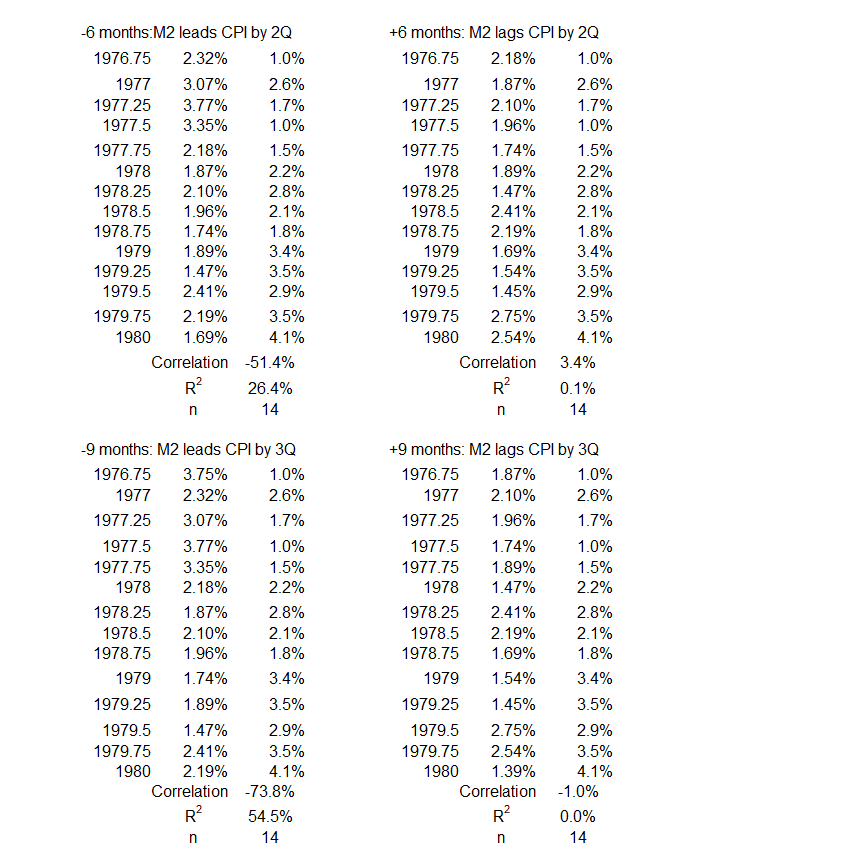
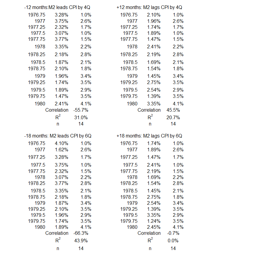
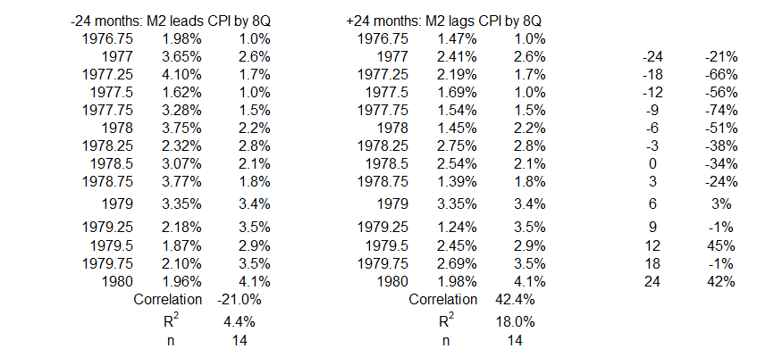
1Q 1977 – 1Q 1980

Figure 10. M2 Money Supply and Inflation 4Q 1976 – 1Q 1980

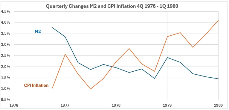
Figure 10 shows M2 money supply changes in a downtrend. CPI inflation changes are in an uptrend.

Figure 11. Quarterly Changes in M2 Money Supply (x) vs. CPI Inflation (y) 4Q 1976 – 1Q 1980

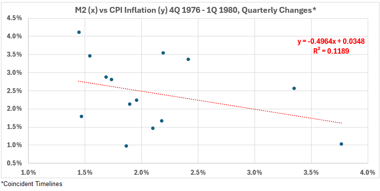
The association between the two variables with coincident timelines is weakly negative. R = –34% and R² = 12%.

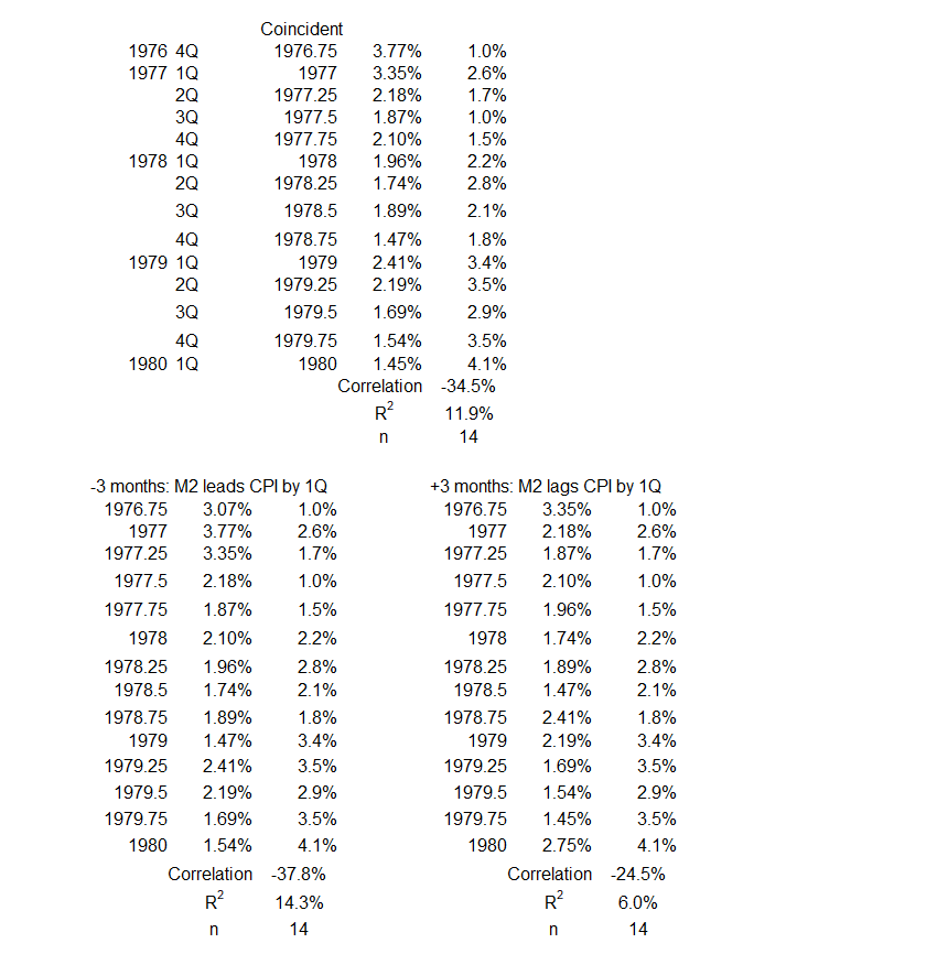
Figure 12. Correlation Between M2 Money Supply and CPI Inflation 4Q 1976 – 1Q 1980

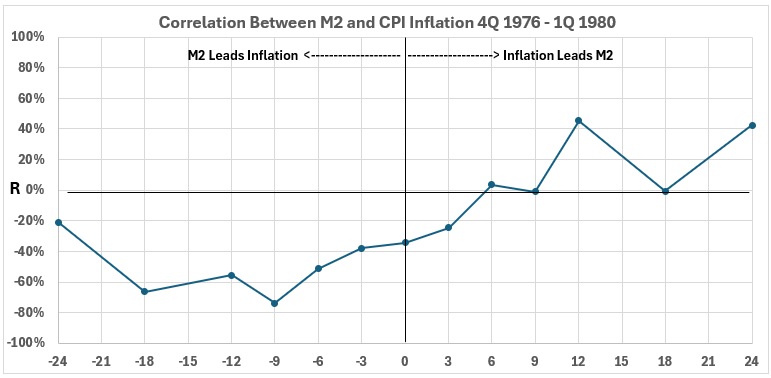
Figure 12 shows that there is no possibility that M2 increases up to 24 months before inflation increases occurred could have been the cause of the inflation changes. (See left side of Figure 12.)

The right side shows limited associations between inflation and subsequent changes in M2. The largest value for R² is 20% (R = 45%), occurring at 12 months.

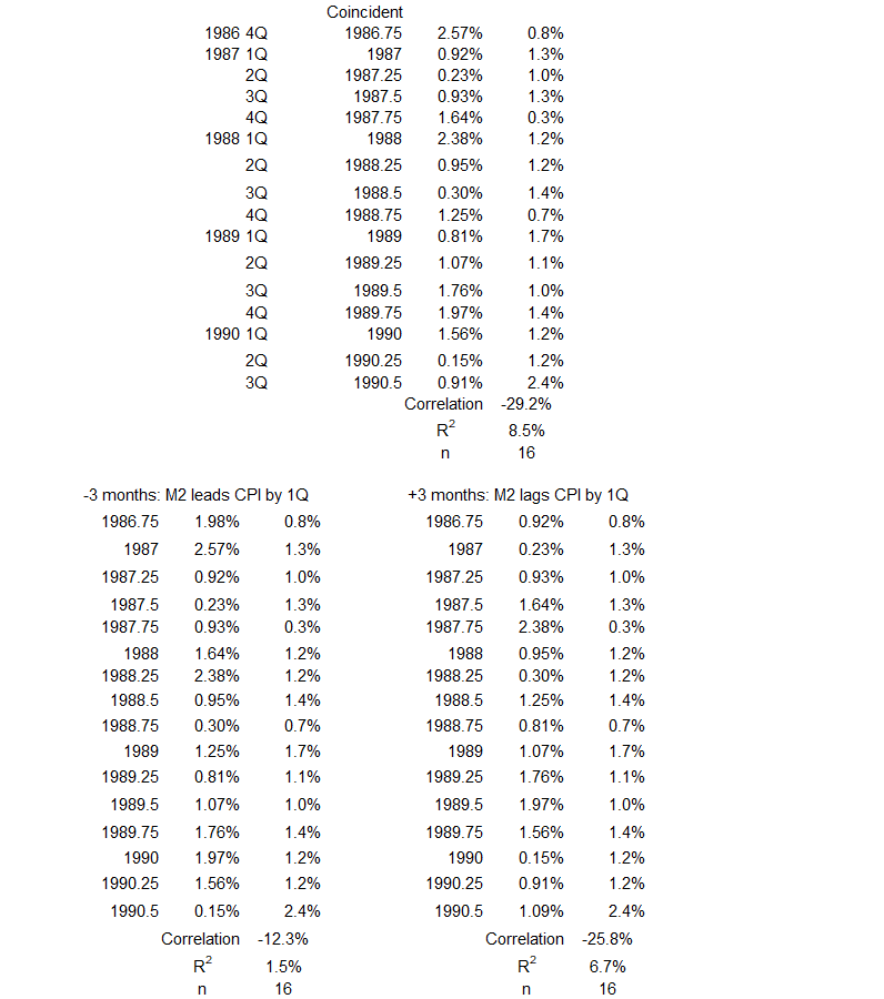
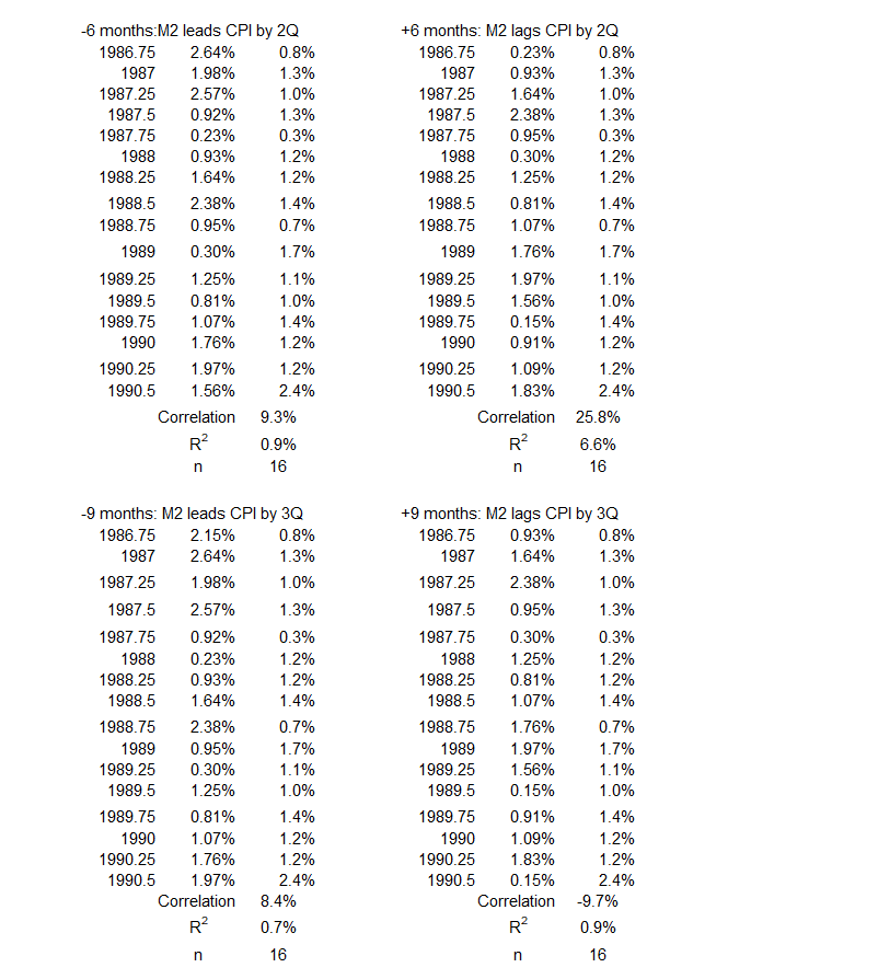
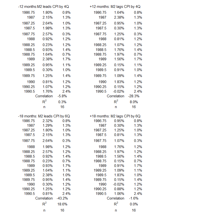
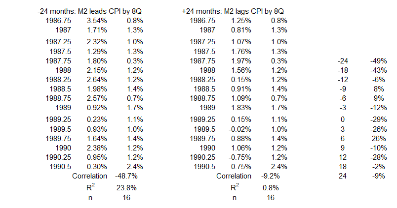
1Q 1987 – 3Q 1990

Figure 13. M2 Money Supply and Inflation 4Q 1986 – 3Q 1990

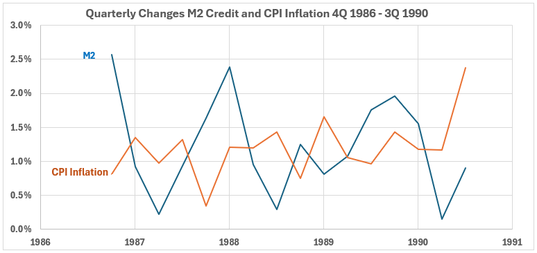
This shows gradual up-trending changes in CPI inflation, while the M2 money supply changes are in a downtrend.

Figure 14. Quarterly Changes in M2 Money Supply (x) vs. CPI Inflation (y) 4Q 1986 – 3Q 1990

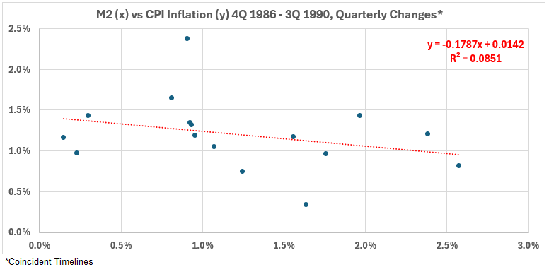
Figure 14 shows a weak negative association between the coincident timeline data sets, R = –29% and R² = 8.5%.

Figure 15. Correlation Between M2 Money Supply and CPI Inflation 4Q 1986 – 3Q 1990

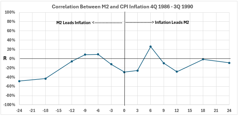
On the left side of Figure 15, there are two positive associations. Both are negligible, with R < 10% and R² < 1%. This indicates that increasing M2 changes could not have caused increasing CPI changes.

The right side shows little opportunity for increasing inflation changes to be associated with later increases in M2 change.

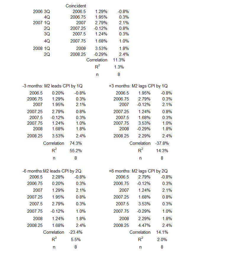
4Q 2006 – 2Q 2008

Figure 16. M2 Money Supply and Inflation 3Q 2006 – 2Q 2008

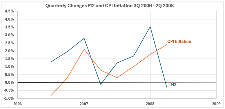
This period covers the end of the housing bubble peak and the start of the stock market decline that was part of the Great Financial Crisis of 2008-09. Here, the changes in CPI are in a gradual uptrend, while the M2 data appears trendless but volatile.

Figure 17. Quarterly Changes in M2 Money Supply (x) vs. CPI Inflation (y) 3Q 2006 – 2Q 2008

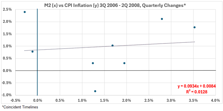
Figure 17 shows a very weak positive association for the coincident timeline data set, R = 11% and R² = 1.3%.

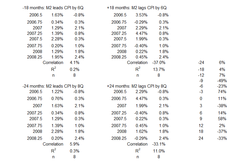
Figure 18. Correlation Between M2 Money Supply and CPI Inflation 3Q 2006 – 2Q 2008

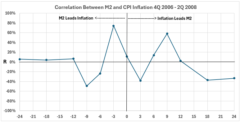
All the data points in Figure 18 show weak or negligible associations with two exceptions. The first exception is at -3 months (M2 change one quarter before a CPI change). Here R = 74% and R² = 55%. This indicates the possibility that M2 change could cause up to 55% of CPI change occurring in the same direction one quarter later.

The second exception is for M2 changes occurring 9 months after CPI changes. Here R = 58% and R² = 34%. This indicates the possibility that M2 changes could result from CPI changes in the same direction three quarters earlier.

Correlation alone cannot determine the extent of cause and effect. Additional information is necessary. One cautionary note for this data set: Both of the largest correlations occur without confirmation from other timeline offset data, which is problematic. It is possible that this period suffers from having a small data set (n=8).

3Q 2009 – 2Q 2011

Figure 19. M2 Money Supply and Inflation 2Q 2009 – 2Q 2011

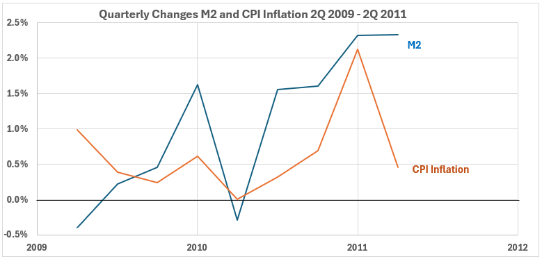
This period starts at the end of the Great Recession of 2008-09. The CPI trend varies from down initially to up, with a steep plunge in the final quarter. The M2 trend is up, interrupted by a one-quarter plunge in 2Q 2010.

Figure 20. Quarterly Changes in M2 Money Supply (x) vs. CPI Inflation (y) 2Q 2009 – 2Q 2011

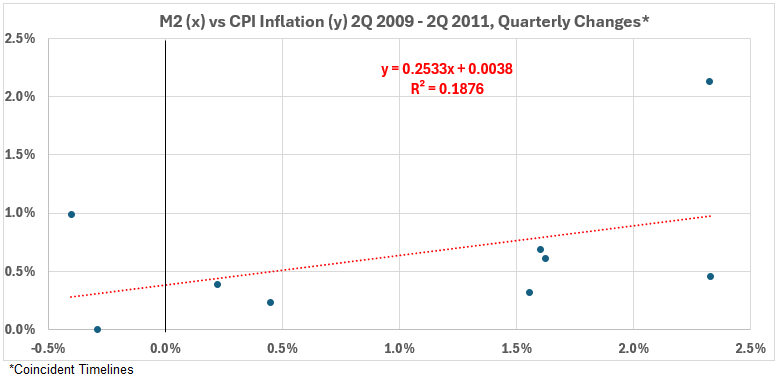
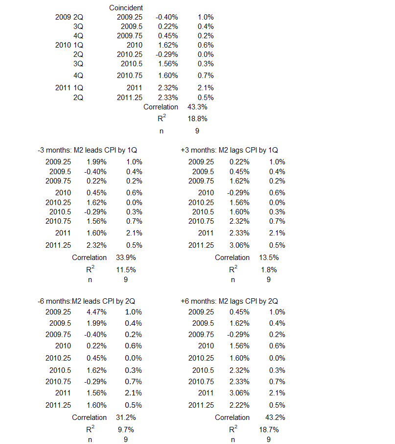
A weak positive association exists for the coincident timelines data, R = 43% and R² = 19%.

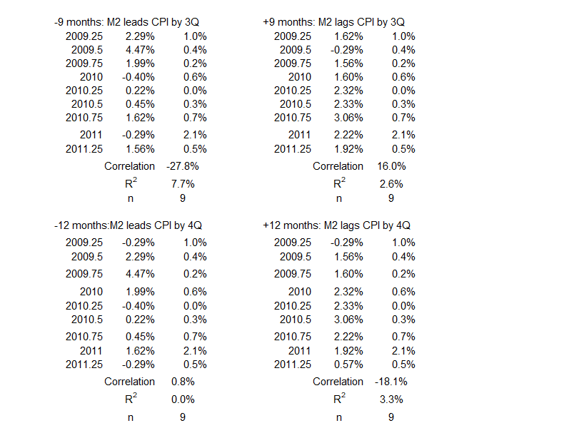
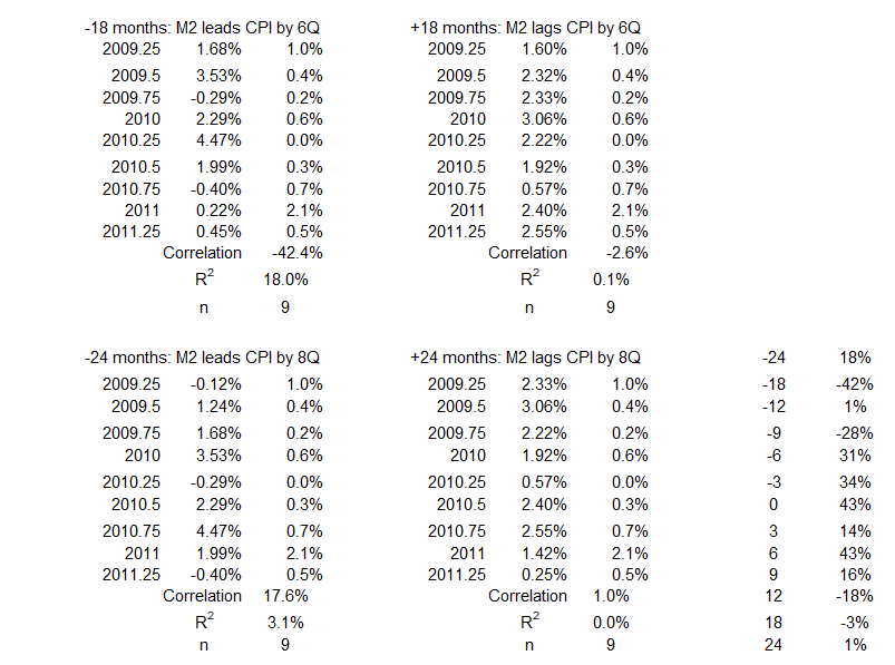
Figure 21. Correlation Between M2 Money Supply and CPI Inflation 2Q 2009 – 2Q 2011

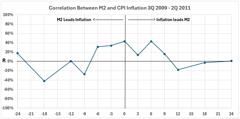
A weak positive association exists for M2 changes occurring coincidentally and 3-6 months before CPI changes in the same direction (Left side of Figure 21). This indicates that up to 20% of CPI changes could be caused by M2 changes in the same direction in the previous six months. However, additional information is needed to determine how much of that 20% possibility is real.

The right side of Figure 21 shows R = 43% and R² = 19% for M2 changes occurring 6 months after CPI changes in the same direction. As for Figure 17, this is not supported by any adjacent timeline offsets, which is concerning. As in the previous case, the results may be problematic due to the small data set size (n=9).

2Q 2020 – 2Q 2022

Figure 22. M2 Money Supply and Inflation 1Q 2020 – 2Q 2022

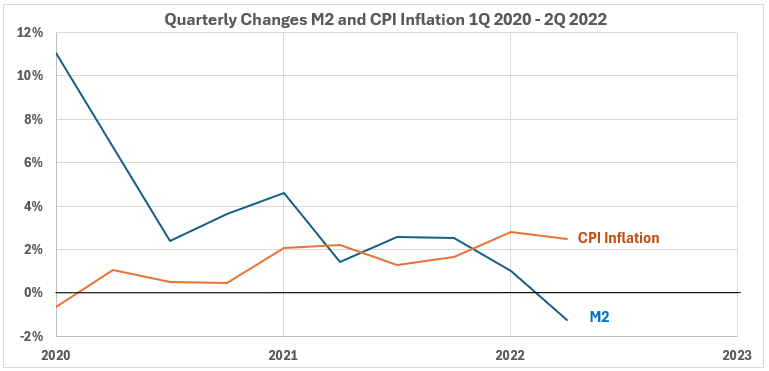
During this period, changes in M2 were in a strong downtrend, while changes in CPI were in a modest uptrend.

Figure 23. Quarterly Changes in M2 Money Supply (x) vs. CPI Inflation (y) 1Q 2020 – 2Q 2022

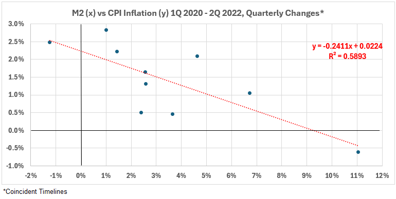
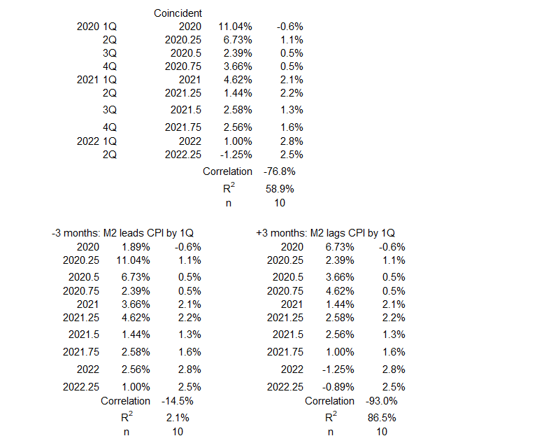
There is a strong negative association for the concurrent timeline data sets. R = –77% and R²= 59%.

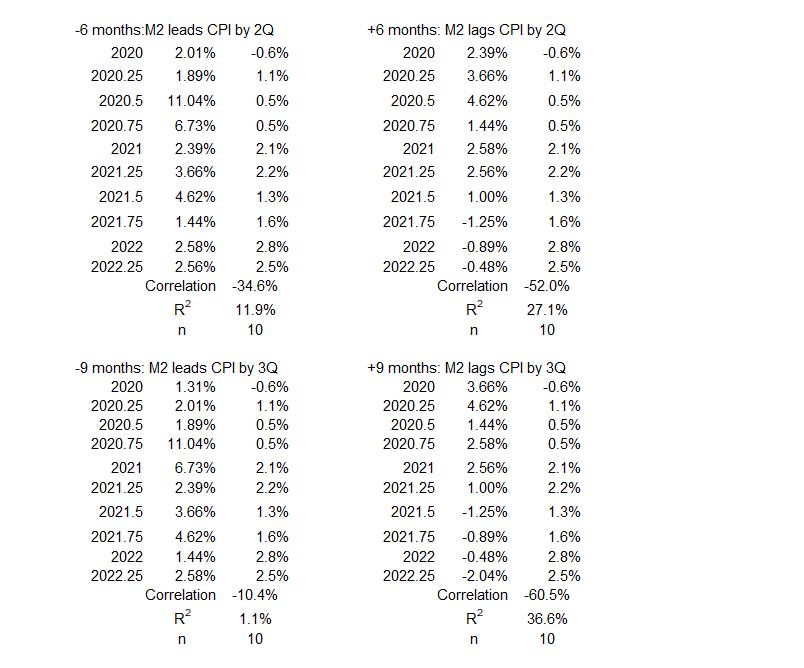
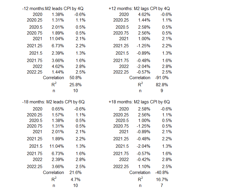
Figure 24. Correlation Between M2 Money Supply and CPI Inflation 1Q 2020 – 2Q 2022

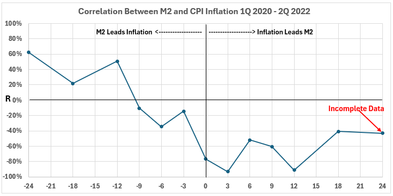
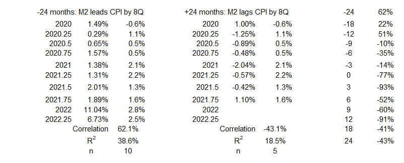
A possibility exists that M2 increases could contribute to CPI increases one to two years later. The two largest R values (-24 and -12 months) are 62% and 51%. This indicates a moderate association with R² values of 38% and 26%. As we have cautioned before, the association only indicates the maximum causation factor, which could be as small as zero, depending on additional information.

The right side of Figure 24 indicates that the only possible changes in M2 after preceding inflation changes would have to be in the opposite direction.

Conclusion

The results of this analysis are surpassing based on the widely perceived belief that increases in money are a significant factor in producing inflation. Of the eight inflation surges studied, only two showed the possibility that increases in the M2 money supply could contribute more than 16% of the subsequent increases in CPI inflation. Four of the inflation surges had 0-5% possible contributions from increases in the money supply to increased subsequent CPI changes.

The two inflation surges with more than 16% possible contributions from increased M2 were in 2006-2008 (up to 55% contribution possible) and 2020-2022 (up to 38% contribution possible).

The three inflation surges where there were no possible contributions by M2 to increases in CPI were 1972-1974, 1977-1980, and 1986-1990.

Note: Possible contributions of M2 to CPI are given as an upper limit based on the correlations determined. Additional information is needed to determine how much of the possibility is realized. Without additional information, the causation could be anywhere from zero to the R² value found.

The data for timeline offsets with CPI changes occurring before M2 changes gives even less definitive information than for the reverse offsets discussed above. There is only one notable result: the 2020-2022 inflation surge. There, the associations indicate that CPI inflation changes are followed by M2 money supply changes in the opposite direction. That makes no sense in reality. Why and how should increases in inflation produce decreases in M2? Why and how should decreases in inflation produce increases in M2? This is almost certainly an example of coincidental associations not related in any way to cause and effect.

Further conclusions will be discussed after we have the data for the deflationary surges and the periods with more stable inflation for the 1952-2011 period. More results there next week.

Appendix

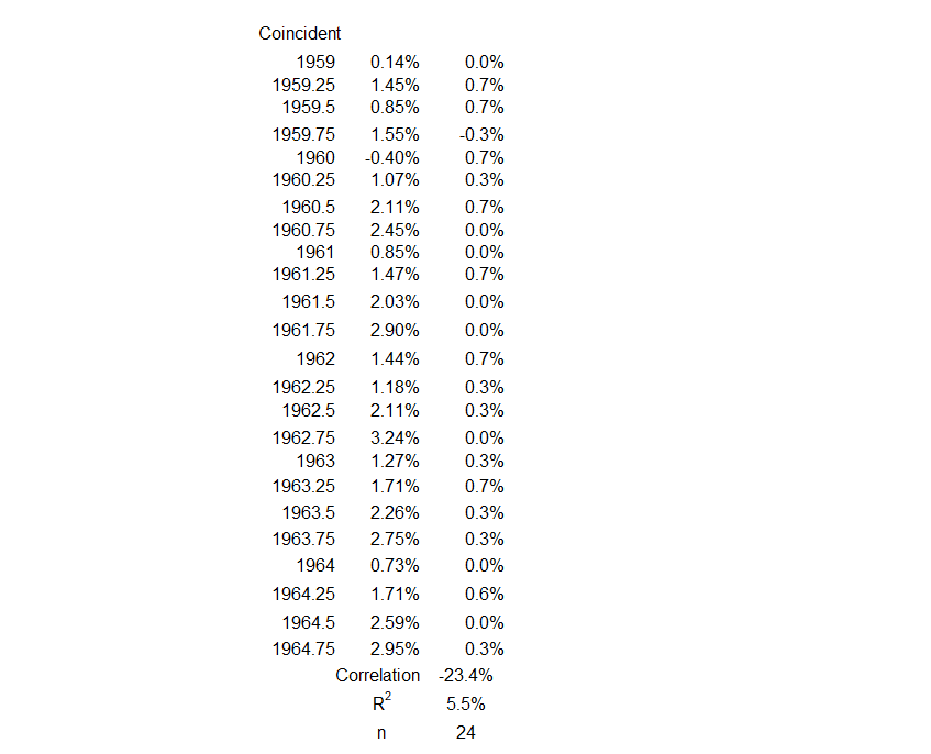
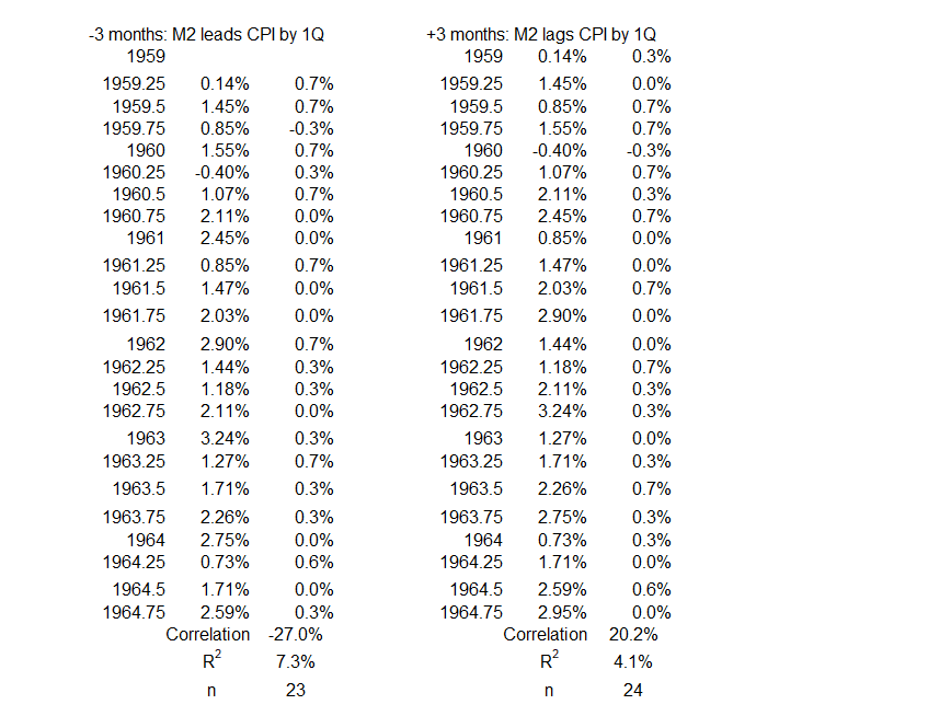
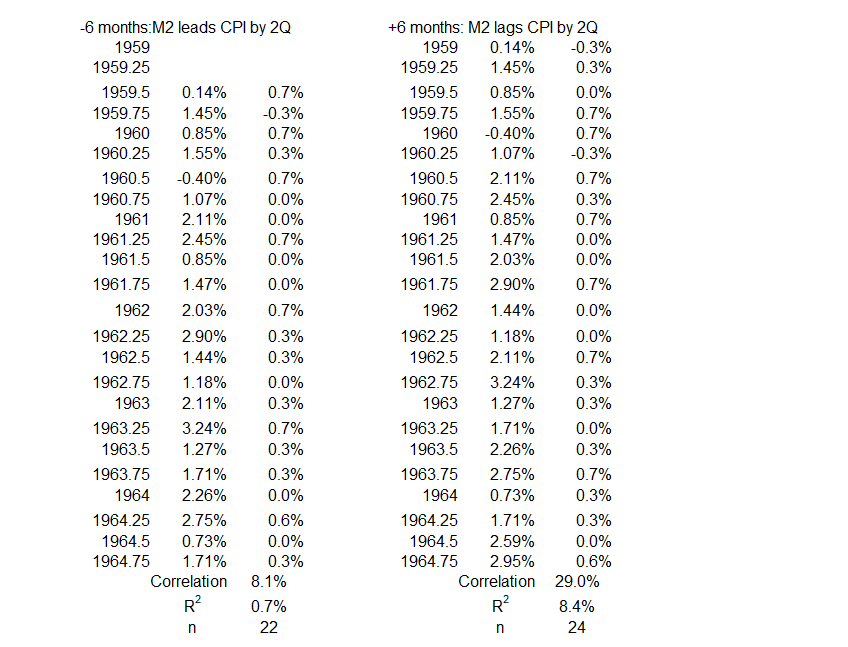
Below are the data sets for each period of surging inflation. They come from the tables of timeline alignments¹(M2 Money Supply and Inflation, Part 1).