For the past several months, we have examined what the U.S. data has to say about the relationships between deficit spending by the federal government and inflation, as measured by the Consumer Price Index (CPI). This post will summarize these results and discuss what they mean.

Image by Gerd Altmann from Pixabay
Introduction
The major objective of this work has been to look for time variation patterns in the correlation between deficit spending and inflation. The primary conclusion of the work is that there are no such patterns. However, there are significant variations in the correlations over time, but the variations appear to be more random than patterned.
A secondary, but almost as important, objective was determining to what extent cause-and-effect relationships might exist between government spending and inflation. There has been consideration of this in the previous articles in the series, but that will be examined in more detail in this piece.
Note: This series of posts has been like entries in an engineering or research notebook. Later articles have made corrections and changes to what appeared in earlier articles. The goal of this article is to summarize the end results and eliminate confusion that might arise from following the work only from Part 1 to Part 15. (For a list of the posts in this series, see the Appendix.)
Proposed Relationship between Federal Government Deficit Spending and Consumer Inflation
The hypothesis we are testing is that inflation depends on federal government deficit spending in a linear manner, expressed in the following equation:
I = mS + b
where
I = Change in CPI (the Consumer Price Index)
S = Change in U.S. Deficit Spending
The two constants, m and b, define the relationship of y, the dependent variable, to x, the independent variable. By writing the relationship in this way, we imply that CPI (y) depends on deficit spending (x). But this is a mere formality because the equation can be rearranged:
S = m’ I + b’
where
m’ = 1/m
b’ = -b/m
We could just as well write the equivalent equation implying that deficit spending depends on inflation without affecting results and conclusions.
We will be looking at correlations in this study. An important relationship to remember is that m is the slope of the line defined by the data points (x,y). If the slope is positive y increases as x increases, which is the characteristic of a positive correlation (correlation coefficient R is positive). If the slope is negative, then the correlation coefficient is negative.
The inflation data for this study were obtained from the Federal Reserve Economic Data for the Consumer Price Index1 for the years 1913-2022, and from the United States Bureau of the Census2 for the years 1792-1912.
The federal government spending data was obtained from the U.S. Department of the Treasury, Historical Debt Outstanding.3
Note on the definition of deficit spending
When there is a deficit, the government spends more than it receives in revenues. Conversely, the government deficit is negative when there is a surplus, ie, the government gets more money than it spends. We have calculated government spending from Historical Debt Outstanding (1791-2022). The calculation is simply
Deficit or Surplus for Year n = National Debt for Year n – National Debt for Year (n-1)
This defines a deficit to be positive and a surplus as negative. This is an appropriate definition since we want to examine the correlation between federal deficit spending and increased inflation. It is possible to look at correlations between increasing negative values of one variable and increasing positive values of another, but that creates negative correlations to confirm what one is looking for. That complicates the discussion.
Attempts to Find Patterns in Long-Term Data Sequences
When this work was started, we hoped to find some consistent patterns in the time-variation of the correlation between federal government deficit spending and consumer inflation (CPI).
We first looked at data from 1793-2022.4 A problem with these time series was that the fiscal data was recorded for fiscal years, while the inflation data was for calendar years. Those two calendars coincided only from 1793-1841. From 1842 on, the two, calendars differed, with the fiscal year being July 1 to June 30, 1841-1975, and October 1 to September 30, 1977 to date. The fiscal year 1976 had five quarters to bridge the calendar change.
From 1913 forward, inflation data has been recorded monthly. This provides data that can be aligned on the calendar with the fiscal year dates.5 It was hoped that the more precise data would enable timeline offsets to be used to identify which came first: spending or inflation. While some very qualitative conclusions seemed reasonable, no systematic patterns of possible cause and effect were evident, even with the more precise data timelines.6,7
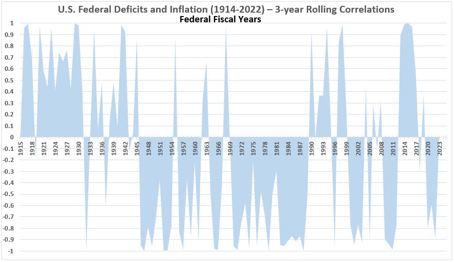
We looked at the time variation by plotting the 3-year rolling average of the correlation over the entire 109 years 1914-20227 and at various large segments of the data. No distinct patterns were found; the variation of correlation over time appeared to be random. Figure 1 and Figure 2 are examples of those results.
Figure 1. Federal Spending and Inflation for the Fiscal Years 1914-2022
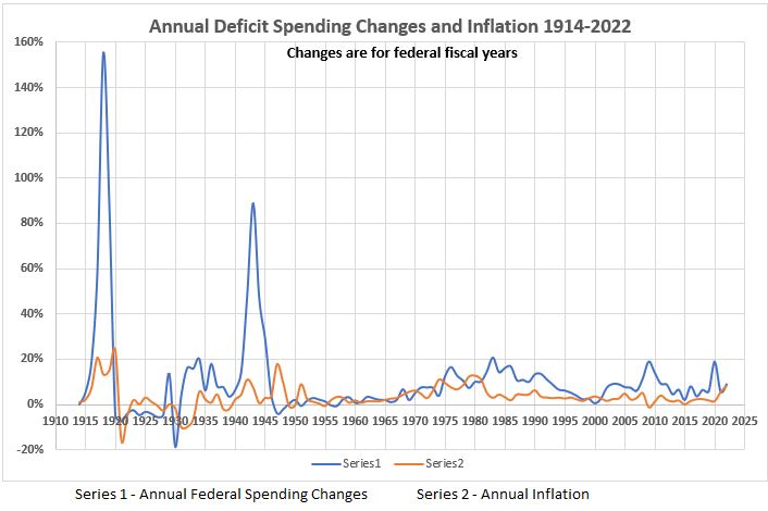
Figure 2. U.S. Federal Deficits and Inflation – Fiscal Years 1914-2022
(Correlation, 3 Month Rolling Average)
The general conclusion at this point was:5
“Another important feature of the graphs is that the more careful timeline alignment of the data has not changed the large number of wild swings in correlation over the 109 year period 1914-2022, compared to our earlier work with less precise data. This seemingly infers that the amount of association between deficit spending and inflation varies widely over relatively short periods of time.”
Periods with and without Inflation Trends
The data has been analyzed using the standard linear regression method.8 The classifications of correlation values used in this study are shown in Table 1.
Table 1. Definitions Regarding Positive Correlations

Definition of Periods with Inflation Trends
Significant inflation trends were defined as those periods of time (fiscal years) when inflation increased or decreased by at least 4% without an intervening countertrend move ≥ 1.5%. The significant trends are identified in Figure 3.
Figure 3. Inflation for the Fiscal Years 1914-2022
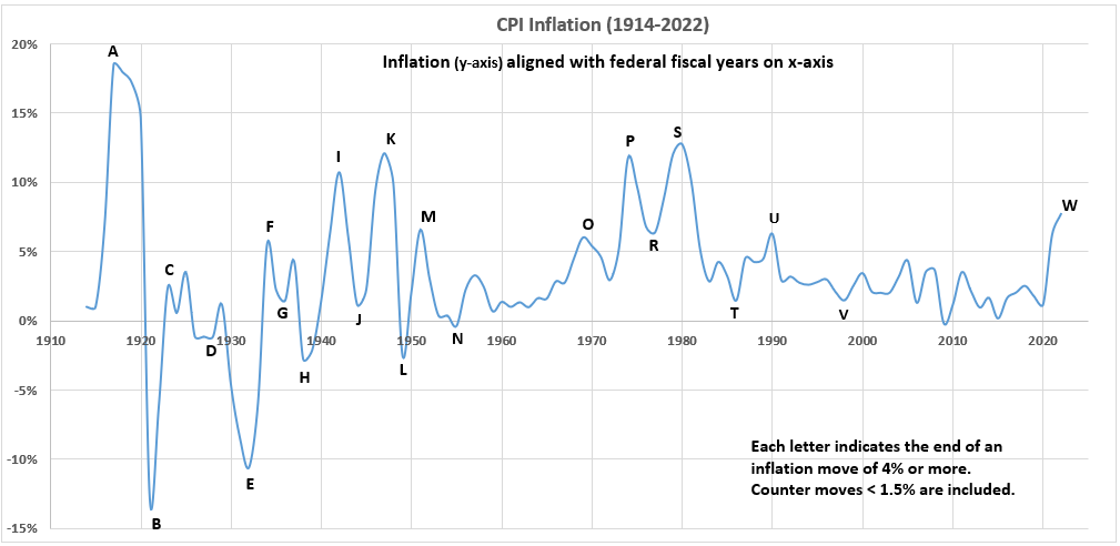
The data for Figure 3 produces the definition of the following inflation periods from 1914-2022:9
- Years belonging to periods in which inflation increased by at least 4% without any countertrend pullback exceeding 1.5%. (11 periods, 38 years)
- Years belonging to periods in which inflation decreased by at least 4% without any countertrend pullback exceeding 1.5%. (11 periods, 37 years)
- The remaining years are not part of a period with significant inflation changes. (6 periods, 34 years)
The summary of the data for these three types of periods follows below.
Significant Inflation Surges
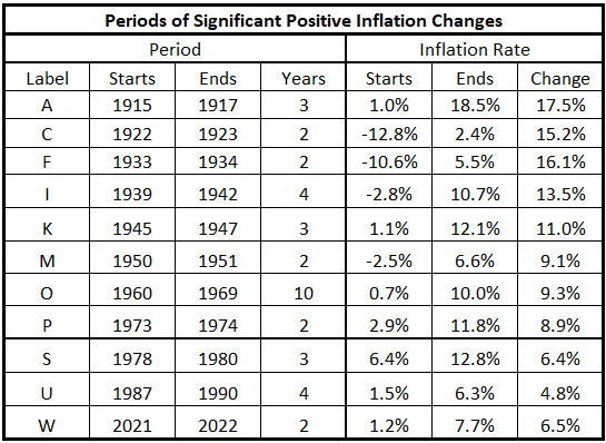
The significant inflation surges from Figure 3 are shown in Table 2.
Table 2. Periods of Significant Increases of Inflation 1914-2022
The analysis of these inflationary periods was presented in three previous posts. 10,11,12
The conclusions, presented previously,12 are shown in Table 3.
Table 3. Correlations for Inflationary Surges and Federal Deficits 1914-2022
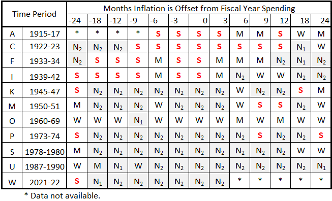
All the significant cells contain a red S, and all the null and negative cells are shaded light gray. This has been done to improve focus when scanning the table.
From Table 3, we draw the following conclusions:
- It is possible that inflation caused deficit spending and deficit spending caused inflation for the inflation surges for all of the inflation periods before World War II (A, C, F, and I).
- The possibilities for either deficit spending causing inflation or inflation causing deficit spending are less after World War II.
- In the post-WWII era, there is the greatest possibility for deficit spending causing inflation for the inflation periods K, M, and P.
- In inflation period O, there is some possibility that inflation caused deficit spending and deficit spending caused inflation.
- Except for period O, there does not appear to be any inflation spike where there is much possibility for inflation to cause deficit spending after World War II.
- There are very small (negligible?) possibilities for causation in either direction for inflation periods S and W, although the possibility for deficit spending causing inflation for W remains with more data.
These conclusions are qualitative. More conclusions are presented in the Quantitative Analysis section near the end of this article.
Significant Deflationary Surges
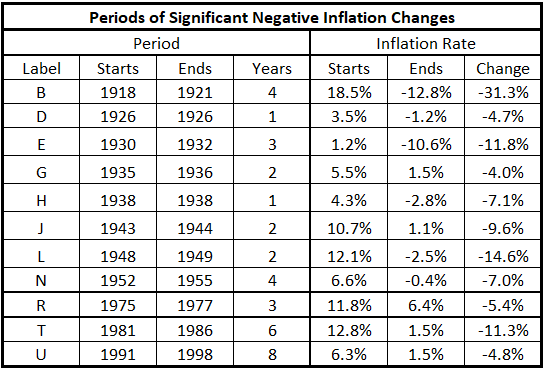
The significant deflationary surges from Figure 3 are shown in Table 4.
Table 4. Periods of Significant Decreases of Inflation 1914-2022
The analysis of these inflationary periods was presented in three previous posts. 13,14
The conclusions, presented previously,14 are shown in Table 5.
Table 5. Correlations for Deflationary Surges and Federal Deficits 1914-2022
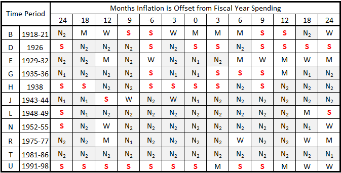
From Table 5, we draw the following conclusions:
- It is possible that disinflation (or deflation) caused deceased deficit spending and decreased deficit spending caused disinflation (or deflation) for the significant inflation declines in all of the declining inflation periods before World War II (B, D, E, G, H). The possibilities are less for time period G (1929-1932) than for the others.
- The possibility for cause-and-effect relationships exists for the World War II period (1943-44) but is relatively small.
- The possibilities for either reduced deficit spending causing disinflation or disinflation causing reduced deficit spending are less after World War II, except for the 1990s.
- In the 1990s, it is possible that deficit spending changes could be major or even dominant causes of disinflation or vice versa.
- In the 1980s, the data suggests that there were no possible direct cause-and-effect relationships between reduced deficit sending and disinflation.
Further discussion of conclusions is presented in the Quantitative Analysis section near the end of this article.
Years not Part of Surges
The analysis of these years9 is summarized in Table 6.
Table 6. Correlations for Inflation w/o Surges and Federal Deficits 1914-2022

From Table 6 we draw the following conclusions:
- It is possible that inflation caused deficit spending, and deficit spending caused inflation for the three time periods before World War II (1924-25, 1927-28, and 1937).
- After World War II, the likelihood that there were cause-and-effect relationships between inflation and federal deficit spending diminished.
- In the 21st century, there is a limited possibility of cause-and-effect relationships between inflation and deficit spending for the years 1999 through 2020.
Limits on Cause and Effect
We have found correlations of federal deficit spending with consumer inflation over 30 specific periods of one or more fiscal years. The correlations found are associations of the two variables in each time period. If a correlation is positive, it indicates the tendency of y to increase when x increases. When the positive correlation is 100% (R = 100%), for that data set, y always increases by a proportional amount when x increases. If R is less than 100%, then one or both of two things have happened:
- y always increased when x increased but not by proportional amounts, and/or
- y has not always increased when x increased.
Note: These associations are mathematical statements for the (x,y) data sets in the analysis. These are not statements indicating that x caused y or vice versa. We need additional information to define cause and effect.
Keeping the above limitation in mind, we do recognize that the square of the correlation coefficient, R2, represents the fraction of y that is mathematically explained by x.
Note: To be more exact, the value of R2 expresses “the fraction of the variance of Y that can be attributed to X.”15
The Maximum Possible Cause of an Effect
Since the correlation determined from a data set is an exact quantity, we can make the following assertion: The value of R2 establishes a limit on the possible cause that x has in producing y. Therefore, if R2 = 50% (0.50), x can cause no more than 50% of y. Other sources must cause at least 50% of y.
But, being repetitive, without additional information, x may cause none of y. Thus the value of correlation alone in establishing cause and effect (CE) is R2 ≤ CE ≥ 0. That means that R2 = 100% (1.00) while being a very significant mathematical statement, has little meaning in and of itself regarding causation: R2 ≤ CE ≥ 0 means 1.00 ≤ CE ≥ 0.
Conversely, while there is uncertain usefulness of a large R2 value, a small R2 is very useful. If R2 = 20%, we infer that 80% or more of the cause of y is something other than x.
The Meaning of the Sign of R
This is very elementary but stated here for completeness. If the correlation coefficient is positive, it means that y has the tendency to increase when x increases. The sign of the slope in the equation y = mx + b is positive, and the magnitude of m indicates the average amount y increases for each unit increase in x. Of course, if b ≠ 0, there is another indication that some other factor than x contributes to y because, when x = 0, b has a non-zero value.
If the correlation coefficient is negative, y has the tendency to decrease when x increases and vice versa.
Note: The value of R2 does not relate to the sign of R. R2 = 100% (1.00) can come from R = 100% or –100%.
How to Interpret a Negative R
As mentioned above, a negative R means that the two variables, x and y, change in opposite directions. This can mean one of two things:
- If the hypothesis is that an increase in x produces an increase in y, then a negative R denies the hypothesis.
- But if there is a possibility that an increase in x can produce a decrease in y, then a negative R confirms that.
In the case of this study, it does not seem reasonable to propose that an increase in deficit spending might cause a decrease in inflation. But, as unreasonable as that might sound, an inverse cause-and-effect relationship is possible without further information. The mathematical observation of a negative R cannot, by itself, indicate that an inverse cause-and-effect relationship does or does not exist.
As always, the assumption is that correlations are circumstantial until proven otherwise. But that assumption does not exclude the possibility of causality.
Quantitative Analysis
The highest associations (correlations) for the various inflationary periods for the 109 years 1914-2022 are shown in Table 7. The highest associations are the maximum possible cause and effect. Of course, in all cases, the minimum possible cause and effect is 0%, as discussed above.
The lead and lag times are in 5 groups in Table 7:
- Inflation leading spending by 18 and 24 months (-18, -24).
- Inflation leading spending by up to one year (-3, -6, -9, -12).
- Inflation and spending aligned to the fiscal year.
- Spending leading inflation by up to one year (3, 6, 9, 12)
- Spending leading inflation by 18 and 24 months (18, 24)
In addition, the data is organized by whether the correlation coefficient is positive (lefthand side of the table), or negative (righthand side of the table).
Table 7. The Highest Correlations for Each Time Period for 1914-2022
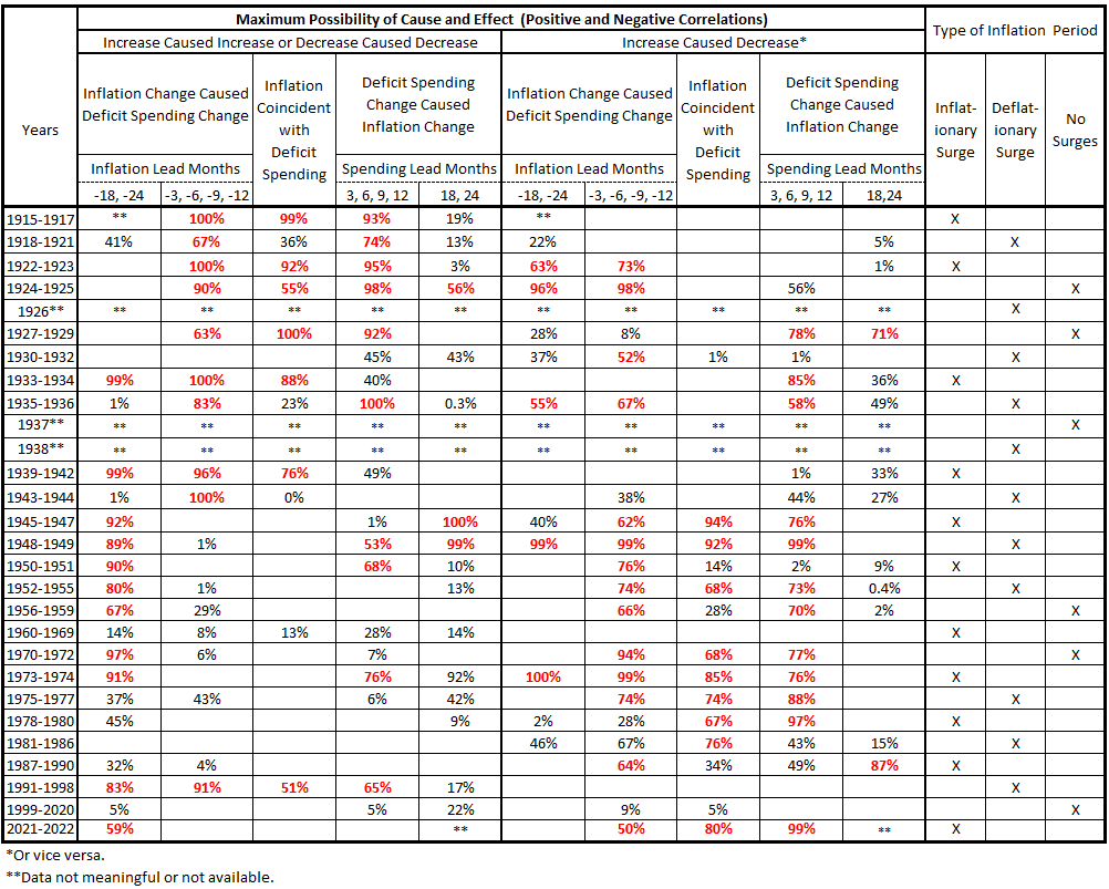
For some time periods, there is no data on one side of the table or another. For example, for 1915-1917, there is no data for negative R. Another example is 1981 to 1986, where there is no data for positive R. Most time periods have data on both sides of the table. Looking at 1922-1923 as an example, we see that there are large R2 values for both positive (100%) and negative (73%) values of R for -3, -6, -9, -12.
What does the data for 1922-1923 mean?
There are four R values, one for each offset of inflation with respect to spending. The data for 1922-1923 has at least one positive R and at least one negative R. The R values in the table are either R2 for a single R or the highest R2 for more than one R. In the case of 1922-1923, there are two negative R values and two positive R values (see Part 13, Appendix 215):
- -12, R = –85.5% —-> R2 = 73%
- -9, R = –79.3% —-> R2 = 63%
- -6, R = 99.8% —-> R2 = 100%
- -3, R = 88.6% —-> R2 = 78%
The R2 values round to 2 significant figures.
Table 7 shows the largest R2 value for each offset grouping. When there are both positive and negative R values in a grouping, the largest for each is shown in the table. Although one might be tempted to dismiss the negative correlation as simply indicating there is no positive correlation, we are not ready to make such an assumption without further information.
Thus, whether increasing deficit spending can cause decreasing inflation or not (or vice versa) should remain an open issue for the time being.
For further analysis, we present the data in Table 7 disaggregated into the following tables.
Table 8. The Highest Correlations 1914-2022 with Substantially Positive Rs
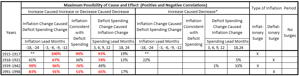
This group of data sets applies to two each inflationary periods and deflationary periods. Except for 1939-1942, there are significant R2 values for both inflation occurring before deficit spending and vice versa. The most plausible explanation is that there is a feedback loop: Once inflation starts, deficit spending increases, and that, in turn, leads to more inflation. The inverse starting order (deficit spending first) can have the same feedback.
Note: The explanation is only valid if inflation causes increased government spending and increased government spending causes inflation. Those are only assumptions at this point. The correlations only show a mathematical association. Cause and effect have not been proven.
Table 9. The Highest Correlations 1914-2022 with More Positive Rs than Negative
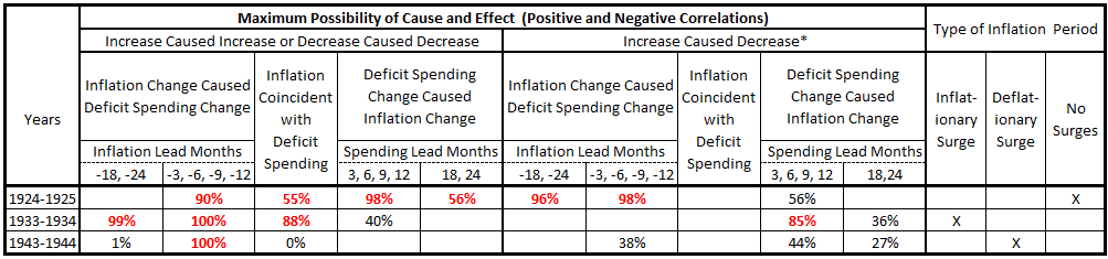
The 1924-1925 period has significant correlations for both positive and negative correlations. How can this be? There may be different levels of cause and effect for positive vs. negative correlations. In other words, either the positive or the negative correlations may be much more circumstantial than the other. Of course, we have no way of knowing that both sets of correlation are circumstantial, as well.
The other two time periods seem to have the positive correlations data stronger than the negative. But the same caveat about circumstantial correlation apply.
Table 10. The Highest Correlations 1914-2022 with Roughly Balanced Positive and Negative Rs
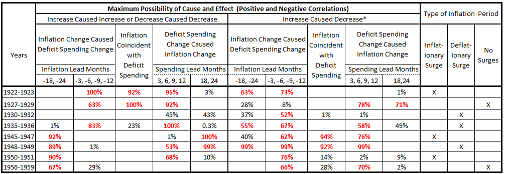
It is interesting that the largest number of time periods fall in this category. This raises a high-level concern that some of the correlations may be substantially circumstantial.
Table 11. The Highest Correlations 1914-2022 with More Negative Rs than Positive
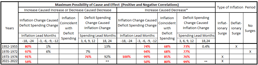
How can increased inflation cause reduced federal deficit spending? How can increased deficit spending cause reduced inflation? It seems the only explanation for this data is a significant amount of circumstantial correlation without cause and effect.
This is a surprising result for the most recent inflation spike associated with the COVID-19 pandemic. Massive government stimulus has been generally considered a major cause for the 2021-2022 inflation spike. This must remain a major red flag for this analysis.
Table 12. The Highest Correlations 1914-2022 with Substantially Negative Rs
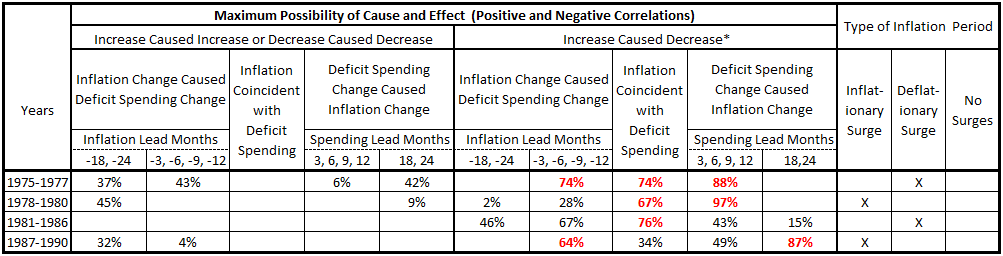
As discussed for Table 11, the only way this data makes sense is if much of the correlation shown here is circumstantial.
Table 13. Correlations 1914-2022 Not Large Enough to be Considered
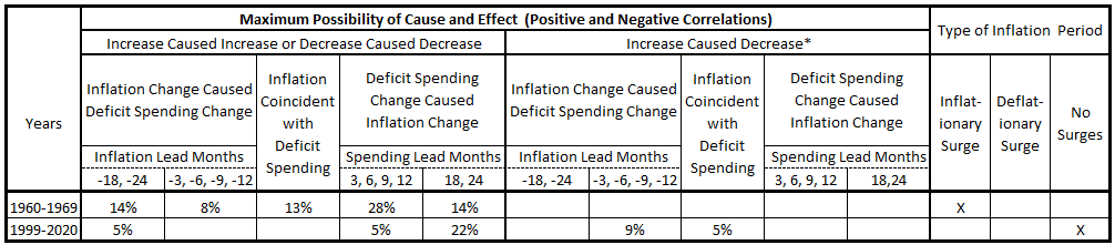
Table 13 indicates there is little chance in these two time periods that there were significant cause-and-effect relationships between federal deficit spending and inflation.
Conclusion
The conclusions of this study are dissatisfying. There appears to be limited opportunity for government spending to have significant cause-and-effect relationships on inflation (and vice versa) in many inflationary and deflationary periods. If this is to be substantiated, there must be other factors for which correlations with inflation are found that could fill in the gaps left by deficit spending.
Among these factors are the following:
- Increased private-sector spending via consumer credit, mortgage lending, non-financial private business credit, and/or financial system credit.
- Wage increases.
- Commodity shortages, especially energy.
- Interest rates.
The next work in this project will look at consumer credit.
Appendices
These appendices are a guide to the posts in the series investigating the correlations between federal government deficit spending and consumer inflation.
Appendix 1
The previous articles in this series are:
Government Spending and Inflation. Part 1 (Inflation and Federal Deficits, 1793-2022)
Government Spending and Inflation. Part 1, Expanded (Inflation and Federal Deficits, 1793-2022)
Government Spending and Inflation. Part 2 (Data Sampling and Data Smoothing Issues)
Government Spending and Inflation. Part 3 (Cause and Effect Issues)
Government Spending and Inflation. Part 4 (Fiscal Year Data)
Government Spending and Inflation. Part 5 (Inflation Leads and Lags with Fiscal Years)
Government Spending and Inflation. Part 6 (Time Variation of Correlation and Graphical Analysis)
Government Spending and Inflation. Part 7 (Statistical Distributions and Correlations 1914-2022)
Government Spending and Inflation. Part 8 (Directionality of Cause and Effect)
Government Spending and Inflation. Part 9 (Directionality of Cause and Effect – Digging Deeper)
Government Spending and Inflation. Part 10 (Inflation vs. Disinflation/Deflation)
Government Spending and Inflation. Part 11 (Inflation Leads and Lags up to One Year)
Government Spending and Inflation. Part 12 (Inflation Surges Analysis, Aborted Due to Errors)
Government Spending and Inflation. Part 13A (Inflation Surges 1914-1942)
Government Spending and Inflation. Part 13B (Inflation Surges 1945-2022)
Government Spending and Inflation. Part 13B – Addendum (Inflation Surge 1987-1990)
Government Spending and Inflation. Part 14A – Deflation (Deflationary Surges 1914-1944)
Government Spending and Inflation. Part 14B – Deflation (Deflationary Surges 1948-2022)
Government Spending and Inflation. Part 15 (Years Not Part of Surges)
Appendix 2
The data in this series are from the following:
1. CPI data from the Federal Reserve1
2. Inflation data from The Statistical History of the United States2
3. Historical Debt Outstanding3
4. Deficit spending rates Inflation and Federal Deficits, 1793-2022
5. Consumer inflation rates Inflation and Federal Deficits, 1793-2022
6. Correlation between deficit spending and inflation with timeline offsets. Inflation Leads and Lags up to One Year, and Inflation Surges 1914-1942 (Appendix A).
Footnotes
1. Federal Reserve Economic Data, Consumer Price Index for All Urban Consumers: All Items in U.S. City Average, Index 1982-1984=100, Monthly, Not Seasonally Adjusted, https://fred.stlouisfed.org/graph/?id=CPIAUCNS,.
2. United States Bureau of the Census (Introduction by Wattenberg, Ben J.), The Statistical History of the United States, Basic Books, New York (1976) pp. 200-202.
3. U.S. Department of the Treasury, Historical Debt Outstanding, Last update October 4, 2022.
https://fiscaldata.treasury.gov/datasets/historical-debt-outstanding/historical-debt-outstanding
4. Lounsbury, John, “Government Spending and Inflation. Part 1, Expanded”, EconCurrents, February 11, 2023. https://econcurrents.com/2023/02/11/government-spending-and-inflation-part-1-expanded/
5. Lounsbury, John, “Government Spending and Inflation. Part 4”, EconCurrents, March 5, 2023. https://econcurrents.com/2023/03/05/government-spending-and-inflation-part-4/
6. Lounsbury, John, “Government Spending and Inflation. Part 3”, EconCurrents, February 26, 2023. https://econcurrents.com/2023/02/26/government-spending-and-inflation-part-3/
7. Lounsbury, John, “Government Spending and Inflation. Part 5”, EconCurrents, March 12, 2023. https://econcurrents.com/2023/03/12/government-spending-and-inflation-part-5/
8. Adler, Henry L. and Roessler, Edward B., Introduction to Probability and Statistics, Fifth Edition, W.H. Freeman and Company, San Francisco, 1972. Chapter 12, pp 195-226.
9. Lounsbury, John, “Government Spending and Inflation. Part 15”, EconCurrents, July 23, 2023. https://econcurrents.com/2023/07/23/government-spending-and-inflation-part-15/
10. Lounsbury, John, “Government Spending and Inflation. Part 13A”, EconCurrents, June 4, 2023. https://econcurrents.com/2023/06/04/government-spending-and-inflation-part-13a/
11. Lounsbury, John, “Government Spending and Inflation. Part 13B”, EconCurrents, June 25, 2023. https://econcurrents.com/2023/06/25/government-spending-and-inflation-part-13b/
12. Lounsbury, John, “Government Spending and Inflation. Part 13B, Addendum”, EconCurrents, July 30, 2023. https://econcurrents.com/2023/07/30/government-spend…art-13b-addendum/
13. Lounsbury, John, “Government Spending and Inflation. Part 14A”, EconCurrents, July 2, 2023. https://econcurrents.com/2023/07/02/government-spending-and-inflation-part-14a-deflation/
14. Lounsbury, John, “Government Spending and Inflation. Part 14B – Deflation”, EconCurrents, July 9, 2023. https://econcurrents.com/2023/07/09/government-spending-and-inflation-part-14b-deflation/.
15. Morin, David, “Probability: For the Enthusiastic Beginner” (p. 294). Kindle Edition.