Previous work has shown that the correlation between US federal government deficit spending and CPI inflation fluctuates widely and wildly over time. Results vary depending on data sample selection. That leads to the present decision to look specifically at each instance of inflation, disinflation, and deflation.

Credit: From a photo by Sam on Unsplash
Introduction
We have made the arbitrary decision to define significant changes in inflation, positive or negative, to be 4% or greater. As shown below in the data section, there are 23 such instances between 1914 and 2022. We allow counter-trend moves <1.5% to occur within each larger move.
Data
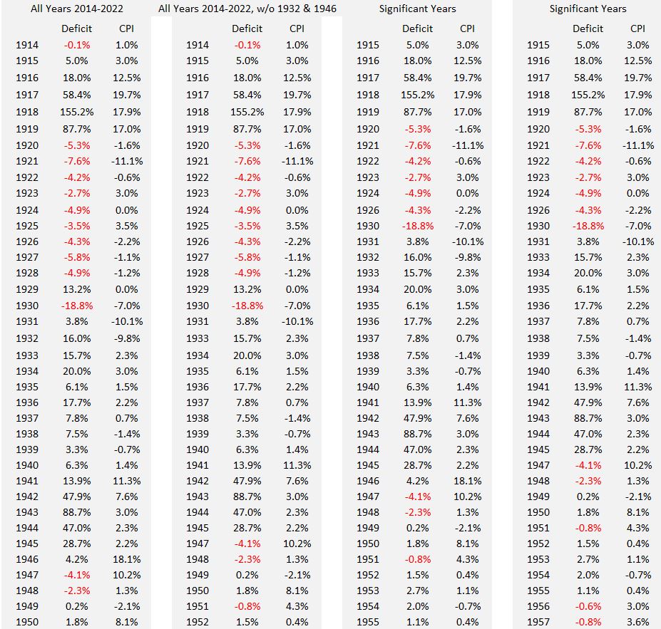
Using the data for inflation from Part 4,1 we have identified 23 significant changes in inflation during the years 1914-2022. These are identified by letters A to X in Figure 1. Note: This is a correction of the inflation graph Figure 1, Part 4.1 The data points for the graph, derived and displayed there, are presented in Table 1.
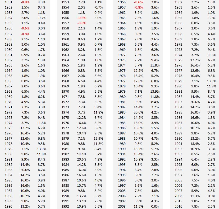
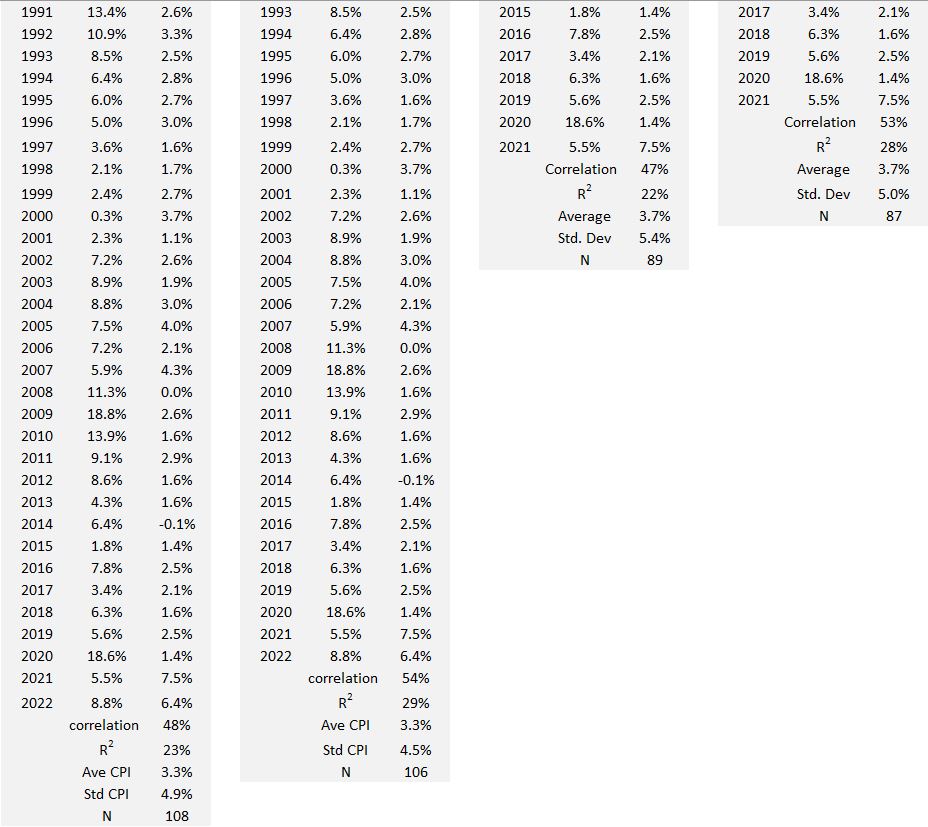
Table 1. U.S. Federal Deficits and CPI Inflation (1914-2022)
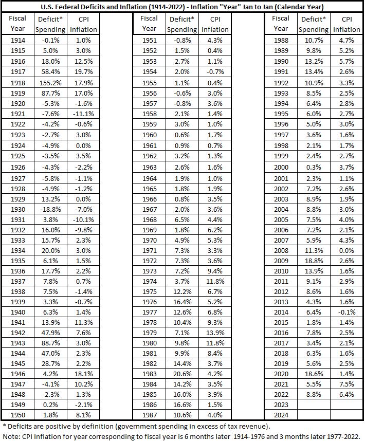
Figure 1. CPI Inflation 1914-2022 with Significant Changes in Inflation Noted
(Each letter identifies the end of a significant move.)
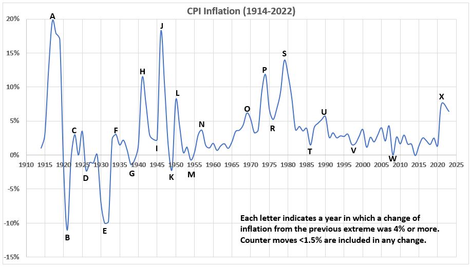
The data derived from Figure 1 is displayed in Table 1 and Table 2.
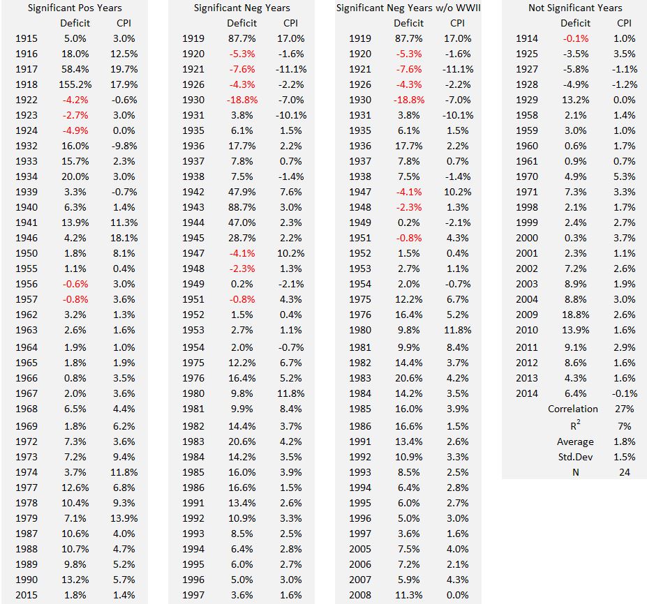
Table 2. Periods of Significant Increases of Inflation 1914-2022
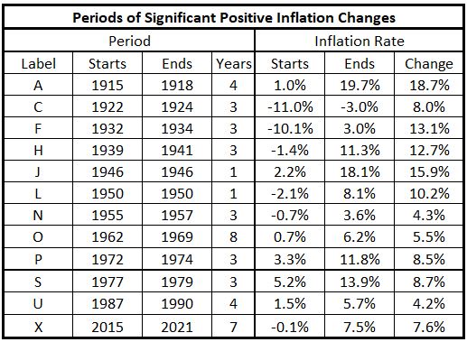
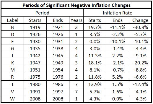
Table 2. Periods of Significant Decreases of Inflation 1914-2022
Analysis
The fiscal years corresponding to the years for the inflation data are six months earlier (July 1 to June 30) for the years 1914-1976, and three months earlier (Otcober 1 to September 30) for 1977-2022. If the first pass analysis here shows promise of revealing any “secrets” about patterns in correlation between deficit spending and consumer inflation, we can return and do the fine tuning of exactly defined alignments between the two data fields. But for now, we will ignore the three and six month misalignments.
Figure 2. Scatter Plot of Inflation vs. Defict Spending for All Data (1914-2022)
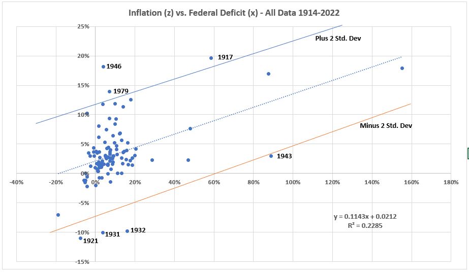
There are 7 data points outside the ± 2σ lines. (Standard deviation = σ.) For 108 data points, the expectation is there should be 5 (5.4 rounded). Therefore, we have omitted the two data points farthest outside ± 2σ (1932 and 1946) and recalculated R2. (See Appendix.) These results are shown in Table 3.
Figure 3. Scatter Plot of Inflation vs. Defict Spending (1914-2022)
Data for Years in Significant Trends
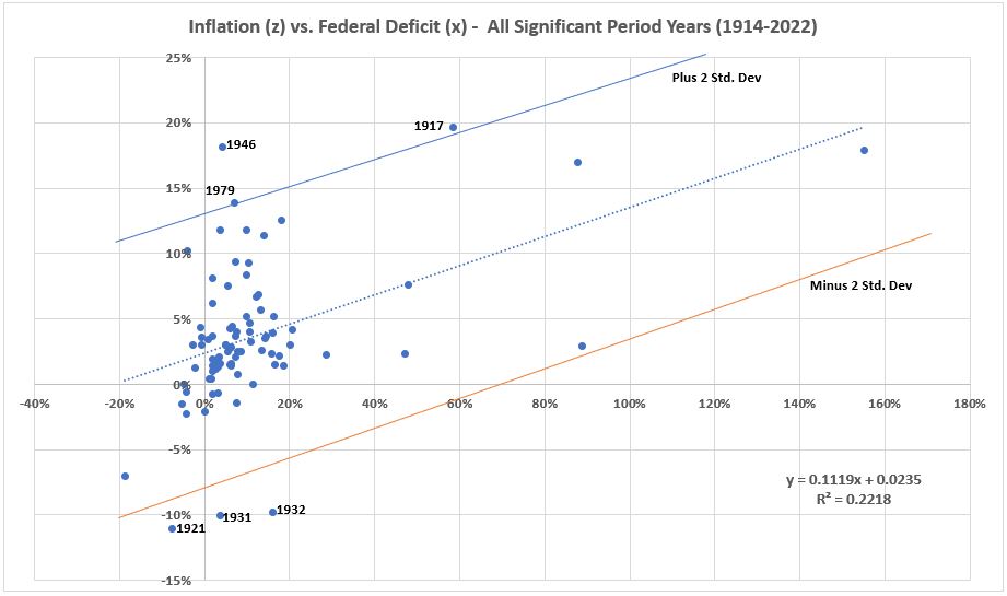
In Figure 3 there are six data points outside the ± 2σ lines. For 84 data points, the expectation is for 4 (4.2 rounded). Therefore, we have omitted the two data points farthest outside ± 2σ (1932 and 1946) and recalculated R2. These results are shown in Table 3.
Figure 4. Scatter Plot of Inflation vs. Defict Spending (1914-2022)
Data for Years in Significant Positive Trends
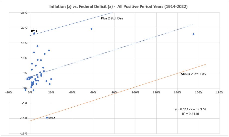
In Figure 4 there are two data points outside the ± 2σ lines. For 43 data points, this is expected (2.15 rounded).
Figure 5. Scatter Plot of Inflation vs. Defict Spending (1914-2022)
Data for Years in Significant Negative Trends
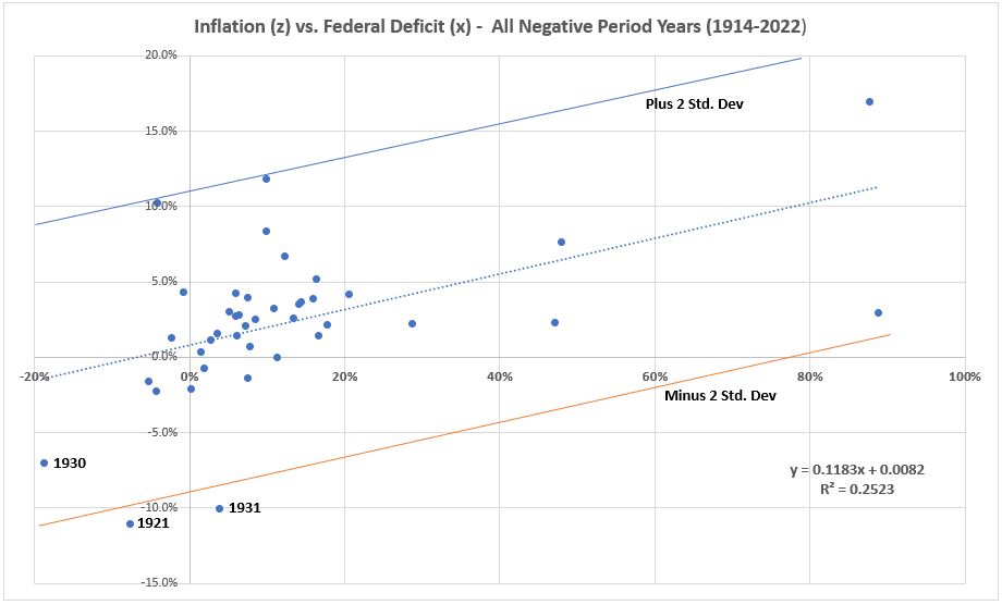
In Figure 5 there are two data points outside the ± 2σ lines. For 41 data points, this is expected (2.05 rounded). However, there is one unusual period in the negative inflation trend series. For the years 1942 – 1945, The U.S. government instituted strict wage and price controls, along with rationing. In Figure 6, a scatter plot of the negative trend data is shown with 1942 – 1945 0mitted.
Figure 6. Scatter Plot of Inflation vs. Defict Spending (1914-2022)
World War II Years Omitted (1942-1945)
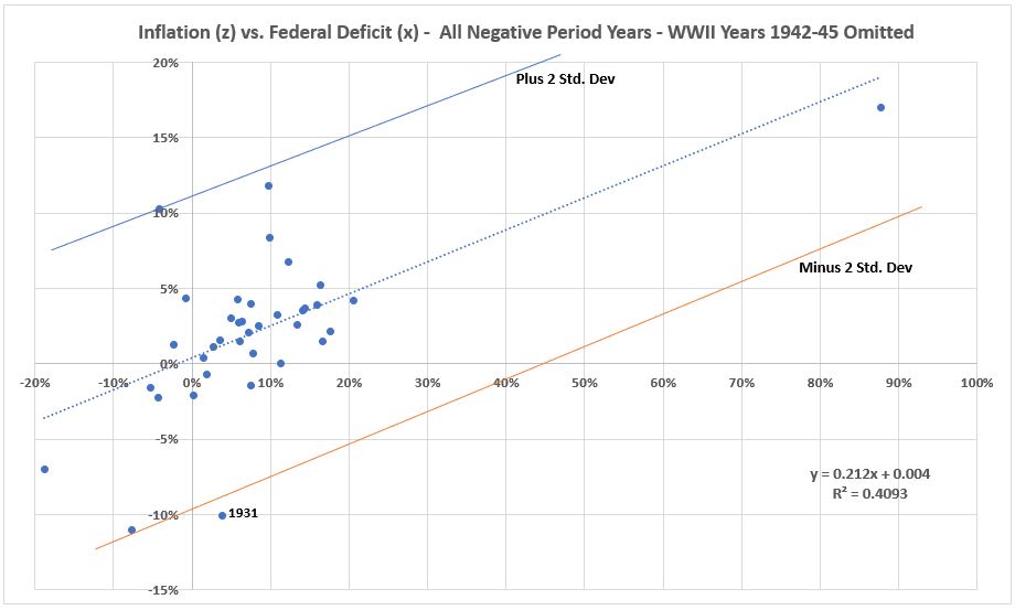
Omitting the World War II years significantly increased the R2 value. There is only one year outside the ± 2σ lines. For 37 data points, this is less than expected (1.85).
Figure 7. Scatter Plot of Inflation vs. Defict Spending (1914-2022)
Data for Years Not in Significant Trends
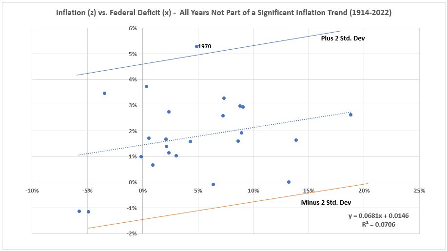
In Figure 7 there is one data point outside the ± 2σ lines. For 24 data points, this is expected (1.2 rounded).
The data from Figures 2 through 7 is summarized in Table 3.
Table 3. Correlation of U.S. Federal Deficits and CPI Inflation (1914-2022)
Trend Analysis
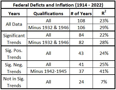
For all of the years included in positive or negative inflation trends, the R2 values all fall in the range of 22% to 29%, except for the ommission of the World War II years when wage and price controls were imposed. The value R2 = 41% for that case indicates that government spending has a stronger association with inflation (disinflation and deflation) than it does when inflation is rising.
Conclusion
The results obtained here are a first pass for this approach because the exact alignment of inflation numbers with federal fiscal years was not done. Results are encouraging. Next week we will proceed with analysis of the data with more carefully aligned timelines.
Appendix
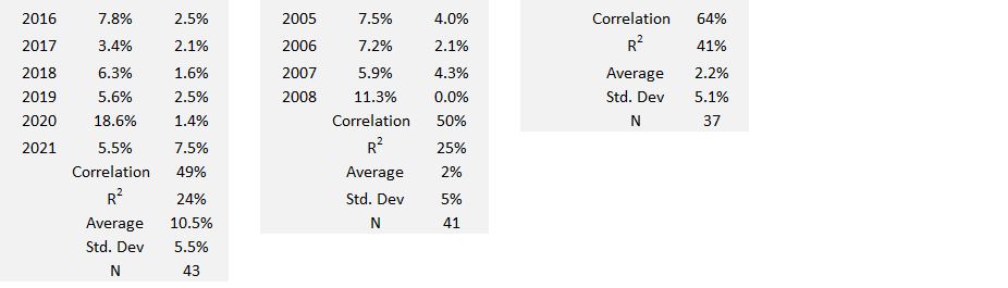
Below are tables of the various data sets used (taken from Table 1) and the summary calculatuioins for each.
Footnote
1. Lounsbury, John, “Government Spending and Inflation. Part 4”, EconCurrents, March 5, 2023. https://econcurrents.com/2023/03/05/government-spending-and-inflation-part-4/.