Government Spending and Inflation. Part 7

This week we examine take a deep dive into what can be learned from examining the unsmoothed data for correlation of deficit spending and CPI inflation.  As before, we are looking at the years 2014-2022.

Credit: From a photo by Carlos Muza on Unsplash.¹

Introduction

Correlation coefficients can be calculated by comparing how data points (in pairs) deviate from the normal distribution functions to which each data series has been fitted.² When one (or both) of the two data series are not well described by a normal distribution (“bell curve”), correlation coefficients may be misleading.³  Outliers (data points far from most of the data set) also confound the meaning of calculated correlation coefficients.  This piece examines the distributions of the two data sets and how the data can be organized to obtain meaningful information about correlations.

Data

The data used this week is the same as shown in Part 5, Table 1.⁴  The only difference here is the correlation numbers shown in the previous table are not included here.

Table 1.  U.S. Federal Deficits and Inflation
Fiscal Years 1914-2022

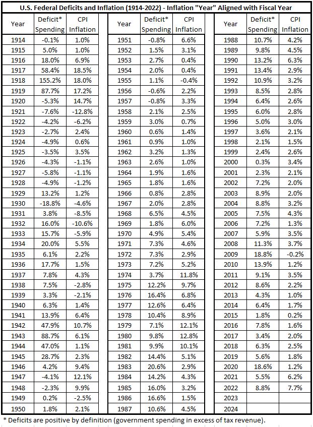
The data in Table 1 has been used to construct⁵ the histograms below.

Distribution of Deficit Spending Data

The data for deficit spending has some clearly identified outliers associated with the peak spending years of the two world wars, shown in Figure 1.

Figure 1. U.S. Federal Deficit Spending 1914-2022

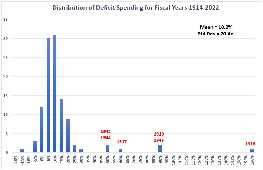
Figure 2. is the same as Figure 1 with the six outlying data points removed from the data set.

Figure 2. U.S. Federal Deficit Spending 1914-2022,
Six World War Years Removed

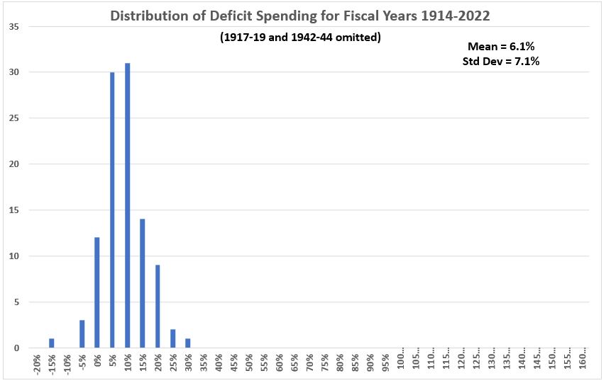
The mean is smaller in Figure 2 and the standard deviation is much smaller, about 35% of the previous value.

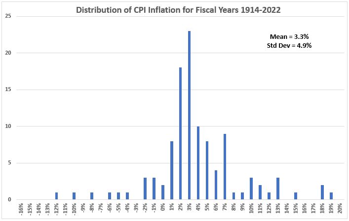
Distribution of CPI Inflation

The histogram in Figure 3 shows that inflation does not appear to have a bell-shaped normal distribution.

Figure 3. U.S. Inflation (CPI) 1914-2022

If we eliminate the six years that were found to be outliers associated with the two world wars , Figure 4 is obtained.

Figure 4. U.S. Inflation (CPI) 1914-2022,
Six World War Years Removed

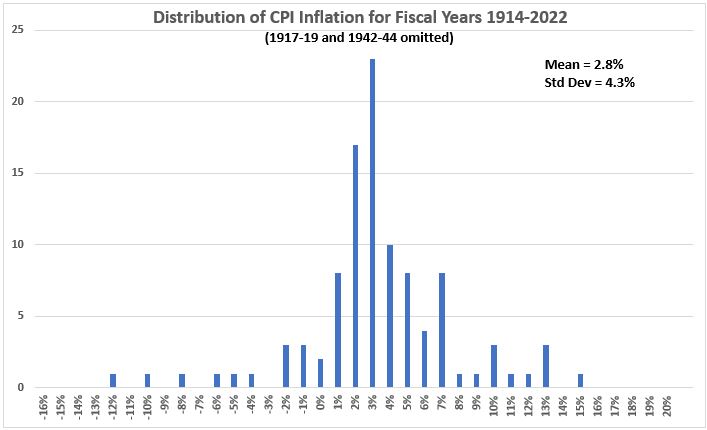
In Figure 4 the mean is reduced by 15% and the standard deviation by 12%, compared to Figure 3.  This is modest improvement in the “tightness” (“narrowness”) of the distribution

We also note that there is one four-year period (1978-1981) of abnormally high inflation due to oil shocks.  Those four years are omitted in Figure 5 (in addition to the six world war years).

Figure 5. U.S. Inflation (CPI) 1914-2022,
Six World War Years & Four Oil Shock Years Removed

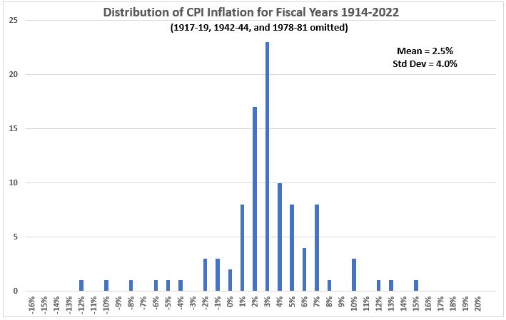
This modestly improves the distribution “tightness” obtained in Figure 4 because the standard deviation decreases slightly (7%) in Figure 5.

Final Adjustment of Deficit Spending Distribution

Figure 6.  U.S. Federal Deficit Spending 1914-2022,
Six World War Years & Four Oil Shock Years Removed

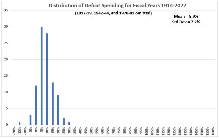
The deficit spending distribution is not “tightened” by removing the additional four years (compare to Figure 2).  Overall, there is not much difference between the distributions in Figure 2 and Figure 6.  The mean is only reduced by 3.2% (6.1% to 5.9%) and the standard deviation is just 1.3% larger in Figure 6.

Analysis

We are now ready to look at correlation.  Using the data in Table 1 and the three distribution conditions in Figures 1-6, correlations have been calculated. (See Figures 7-9.)

Figure 7. Deficit Spending vs. Inflation 1914-2022

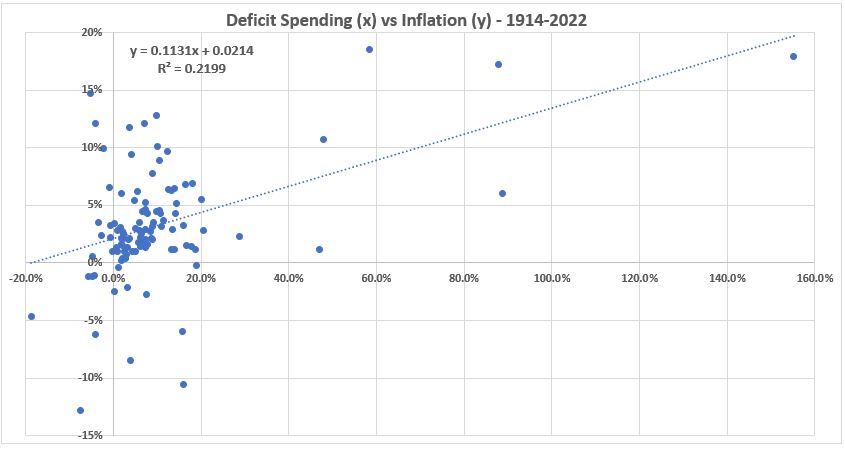
Figure 8.  Deficit Spending vs. Inflation 1914-2022
(1917-19 and 1942-44 Years Omitted)

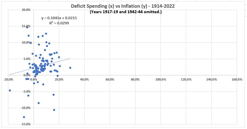
Figure 9.  Deficit Spending vs. Inflation 1914-2022
(1917-19, 1942-44, and 1978-81 Years Omitted)

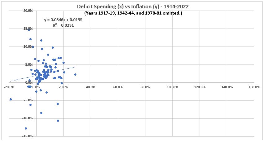
The three figures above show the unexpected result that the correlation between the two data sets declined as outliers to the two normal distributions were removed.  Note:  All three graphs are plotted with the same x,y axes for ease of comparison.

Should we proceed for further analysis with the two full data sets and ignore the “improvement” of removing outliers?  That is an option but we are reminded of the cautionary remark of Freeman et al:³

“The correlation coefficientis useful for football-shaped scatter diagrams.  For other diagrams, r can be misleading.  Outliers and non-linearity are problem cases.”

The letter r above is the correlation coefficient which we have represented by R.

In the pages before the quote above, the authors had shown that normally distributed data displays in a football shape in x,y scatter plots as have been produced above.  In the three graphs above, only Figure 7 for the full data set shows anything with the faintest resemblance to the shape of a football, even though the left end is substantially overweighted with data.

It is prudent to look further at the data to see if there is some way we can work with data sets that are better represented by normal distribution curves.

More than One Distribution

A collection of data may contain more than one distribution.  After the 10 outlier data point were removed, there remained three separate time lines for the data: 1920-1941, 1946-1977, and 1982-2022. What the six data subsets look like when examined for the nature of their distributions and correlations are show in the Appendix.

The six distributions all appear to deviate substantially from the normal curve.  The correlations for each of the three time periods are quite low.  For the time being, at least, we are not pursuing the question of using smaller data subsets for analysis.

Conclusion

The results obtained above indicate that the 108 years of data have a correlation coefficient of 47% (R² = 22%).  This is a significant association between deficit spending and consumer inflation.  None of the segmentations of the data examined yielded any significant associations.  Repeating an oft repeated caution, association doesovide a maximum limit for the portion of causation of one variable on the other.  In other words, if independant information does establish not infer any cause and effect relationship. If such exists it must come from other information. But the R² value does prthat deficit spending does increase inflation, the maximum contribution to inflation from that source is 22%.  That means that, on average over the 108 years, 78% or more of inflation is caused by something other than federal deficit spending.

Of course, without additional information, the amount of inflation caused by deficit spending could still be as low as zero.  So at this point we can state that, if deficit spending contributes to inflation, the amount of that contribution is ≥0% and ≤22%.

Also, there is nothing that we have seen so far indicates causation cannot occur in the oppositie direction.  Inflation might cause increased deficit spending under some circumstances.  If that were to occur, the same limits of ≥0% and ≤22% apply to the amount of increased deficit spending caused by inflation.

Inflation and deficit spending may be mutually reinforcing via feedback loops.  We haven’t yet formulated a model to evaluate how mutual feedback mechanisms could come into play.  Such a model would require dynamic treatment of the time-variation of correlation such as we have attempted in previous parts of this series.  It is hoped that further progress on this may come in future weeks.

Appendix

Let’s look at the as three separate data sets that remain after removal of the six world war years and the four-year 1978-81 oil shock for each of the variables deficit spending and inflation.  The first three graphs below show the scatter plots for the paired data sets.

Figure A1. U.S. Federal Deficit Spending vs. CPI Inflation, 1920-1941

 

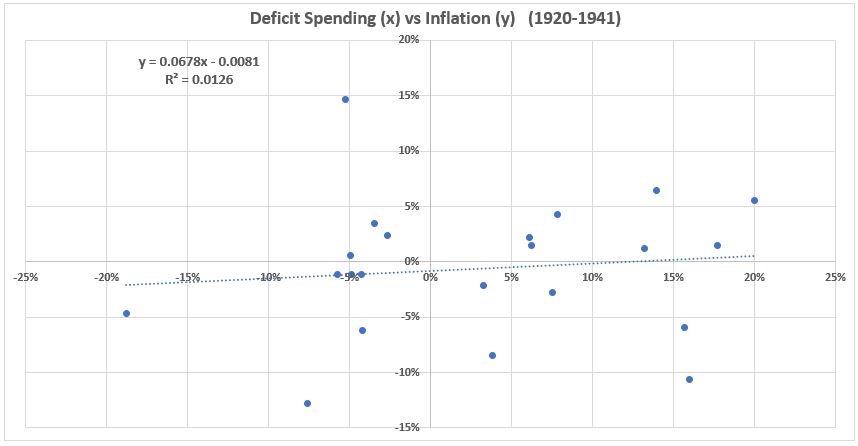
Figure A2. U.S. Federal Deficit Spending vs. CPI Inflation, 1945-1977

 

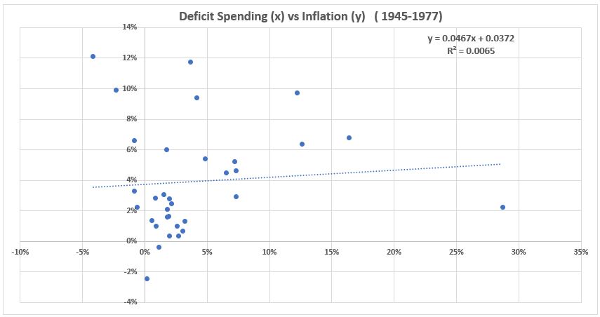
Figure A3. U.S. Federal Deficit Spending vs. CPI Inflation, 1982-2022

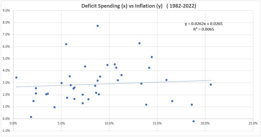
There is little promise of usefulness of the three data sub-groupings.  The R² values are very small ( just above and below 1%).  The most likely reason for this disappointing result compared to the same treatment of the entire data set is that the number of data points in each subgroup are insufficient to represent each entire population.  If quarterly data were available, this hypothesis could be tested.

An alternative explanation is also possible:  While the entire data set for 108 years provides a seemingly satisfactory treatment as a normal distribution, it may be composed of subdata sets that will never each individually follow a normal distribution curve no matter how many measurements are made.  The overall normal distribution behavior of all the data points taken together could therefore be happenstance and not related to the distributions in the component subsets.

In the six graphs below, we see that the distribution histograms have significant deviations from the bell-curve shape of normal distributions.  Again we hypothsize that the number of data points in each subgroup is insufficient to provide an adequate representation of a total population.

Figure A4.  U.S. Federal Deficit Spending 1920-1941

 

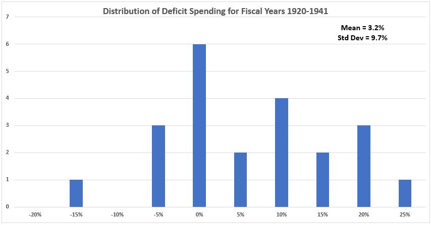
Figure A5.  U.S. Federal Deficit Spending 1945-1977

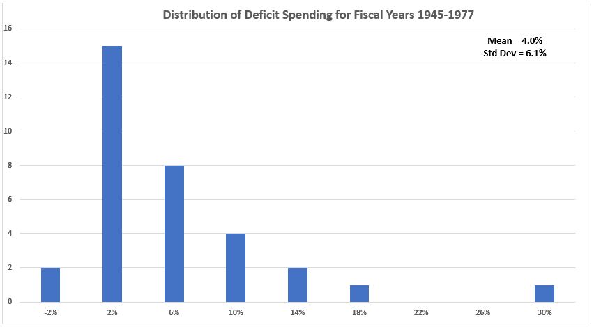
Figure A6.  U.S. Federal Deficit Spending 1982-2022

 

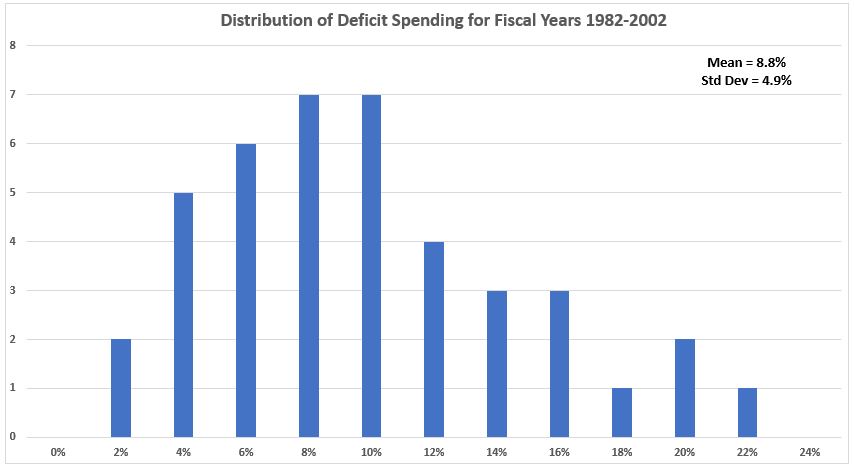
Figure A7.  U.S. Inflation (CPI) 1920-1941

 

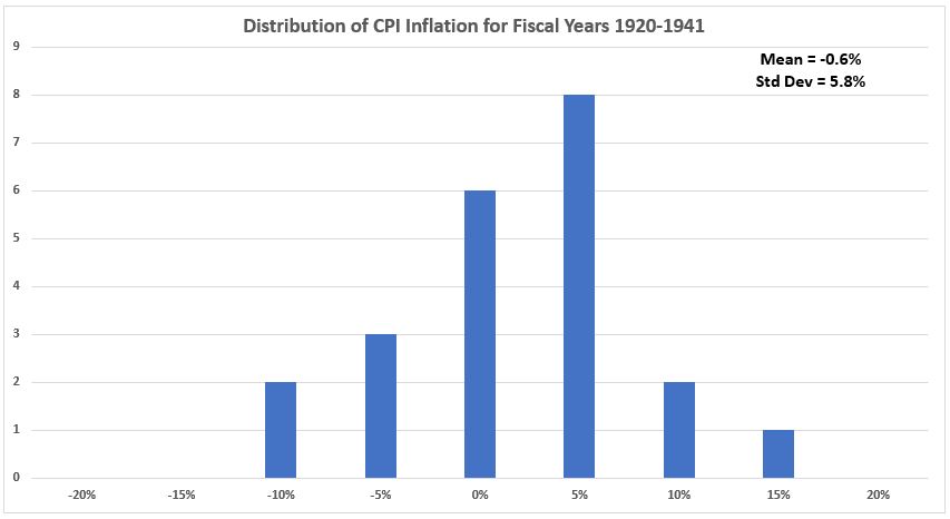
Figure A8.  U.S. Inflation (CPI) 1945-1977

 

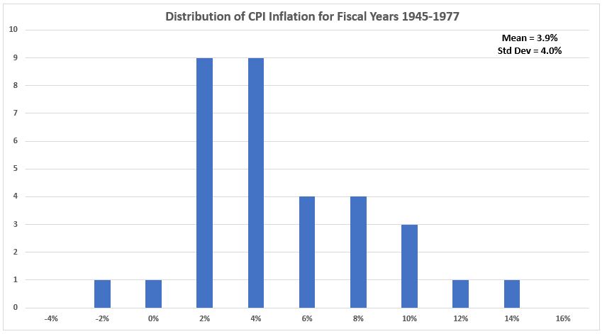
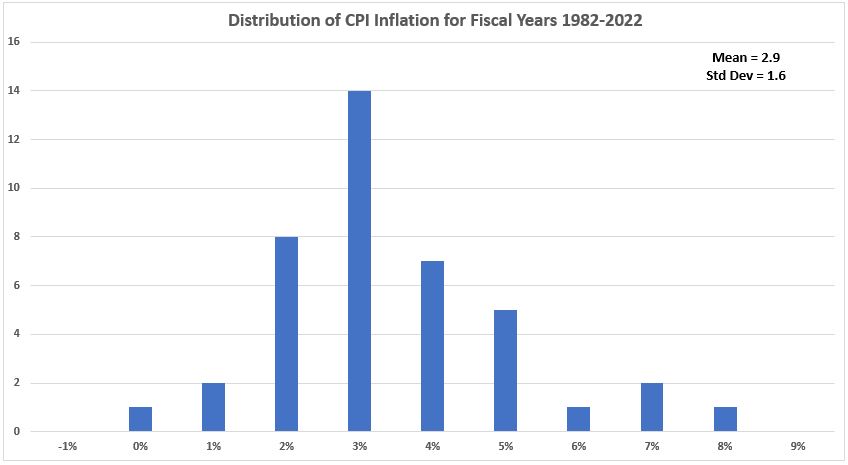
Figure A9.  U.S. Inflation (CPI) 1982-2022

Footnotes

1. Muza, Carlos, Statistics on a laptop, photo, Unsplash, 2016.  https://unsplash.com/photos/hpjSkU2UYSU.

2. Freedman, David, Pisani, Robert, and Purves, Richard, Statistics, Fourth Edition, W.W. Norton & Company (New York) and Viva Books (New Delhi), 2009. See Chapters 8 & 9 for explaination of how normal distributions relate to determination of correlation coefficients.

3.  Ibid, page 147.

4.  Lounsbury, John, “Government Spending and Inflation. Part 5”, EconCurrents, March 12, 2023. https://econcurrents.com/2023/03/12/government-spending-and-inflation-part-5/.

5.  O’Loughlin, Eugene M.F., How to Plot a Normal Frequency Histogram in Excel 2010, National College of Ireland.  YouTube:  https://www.youtube.com/watch?v=UASCe-3Y1to

6.  Lounsbury, John, “Government Spending and Inflation. Part 6”, EconCurrents, March 26, 2023.  https://econcurrents.com/2023/03/26/government-spending-and-inflation-part-6/.