Note: This was posted at 4:24 pm on March 26 with some incomplete sections.  Updating in was completed at 2:52 am March 28.

In previous parts of this discussion, we have made some qualitative observations about relationships involving the correlations between U.S. federal government spending and inflation in the U.S. economy. For the first time in this series, we will move into the arena of quantitative measurements of government spending and inflation correlations.

Credit:  Photo by Mahdi Soheili on Unsplash

Introduction

Previously,¹ we developed graphs that showed the short-term correlations between deficit spending and CPI inflation.  Now we will make quantitative measurements of those graphs.  To do this, we will use the technique of measuring the area under a curve. The areas under the curves in each graph will be calculated using only two geometric shapes that fit all of the data used.²  These two shapes are triangles and trapezoids. Figure 1.  The areas of these two shapes are calculated as shown below in Figure 1.

Figure 1. Triangles and Trapezoids

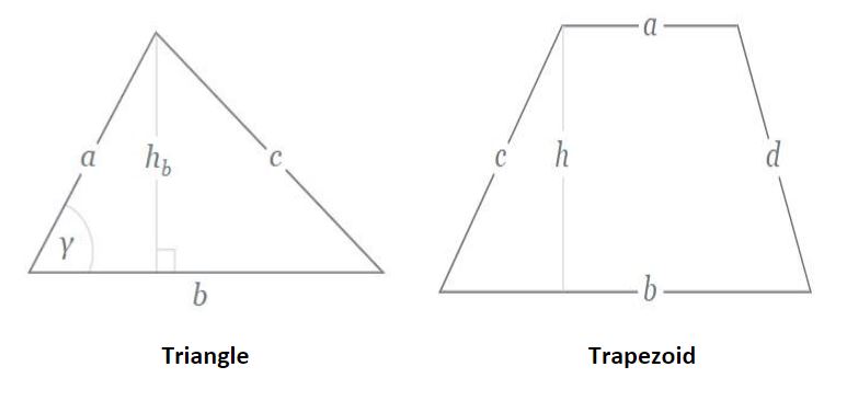
Area of a triangle = h_b b / 2

Area of a trapezoid = h (a+b) / 2

Data and Calculations

Correlation of Inflation Coincident with Deficit Spending

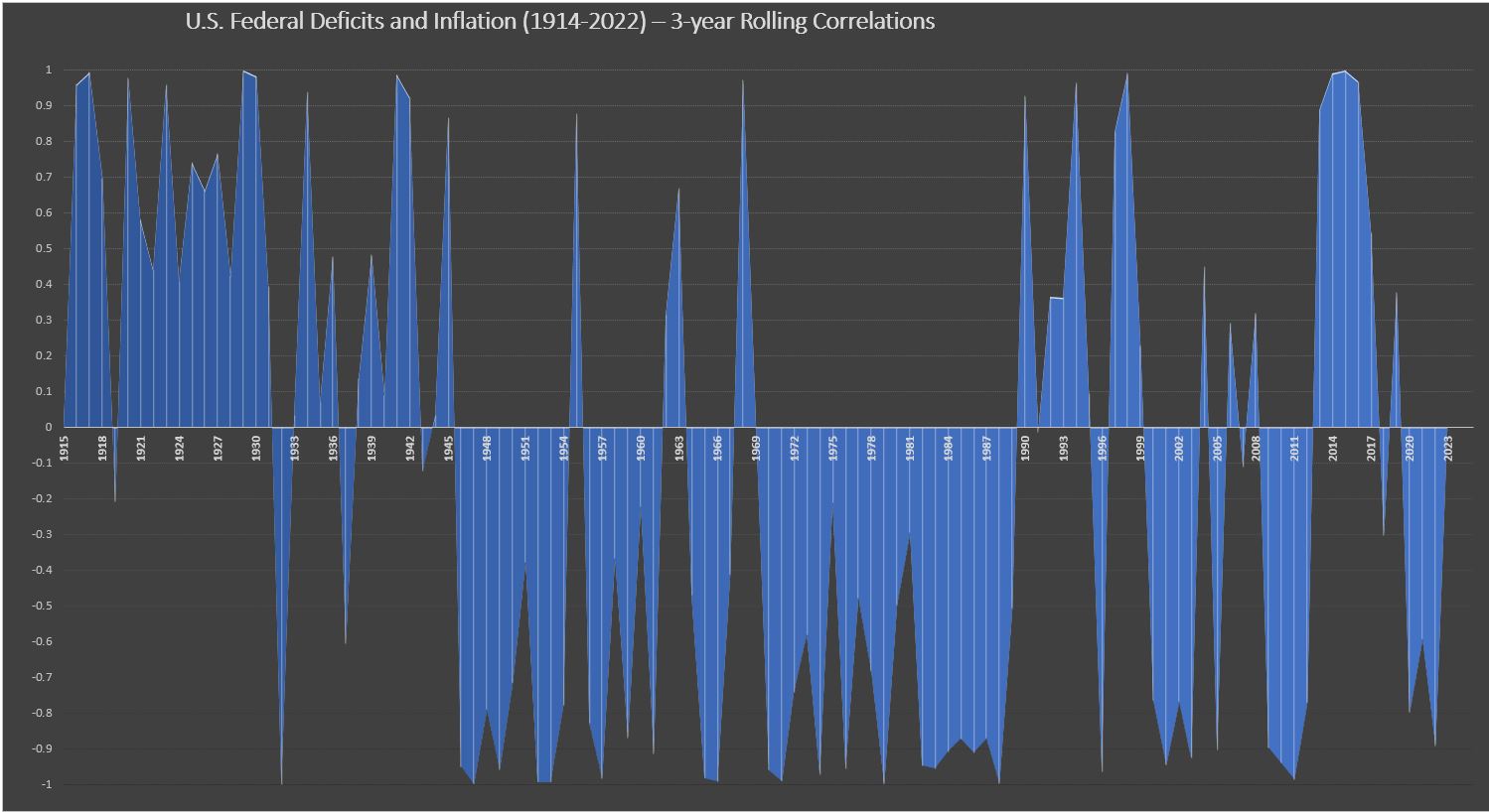
In Figure 2 we have a new presentation of the 3-year rolling average of correlation (Figure 1 in Part 5¹) showing the geometric structures under the curve.

Figure 2.  U.S. Federal Deficits and Inflation  – Fiscal Years 1914-2022
(Correlation, 3-Year Rolling Average)

Click here for larger image in a new window.  Exit new window (back arrow) to return to this page.

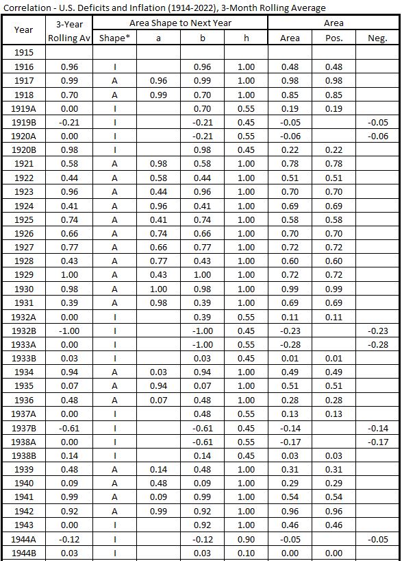
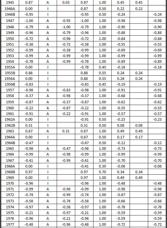
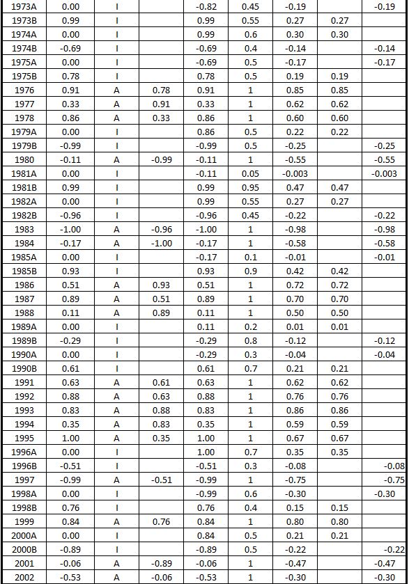
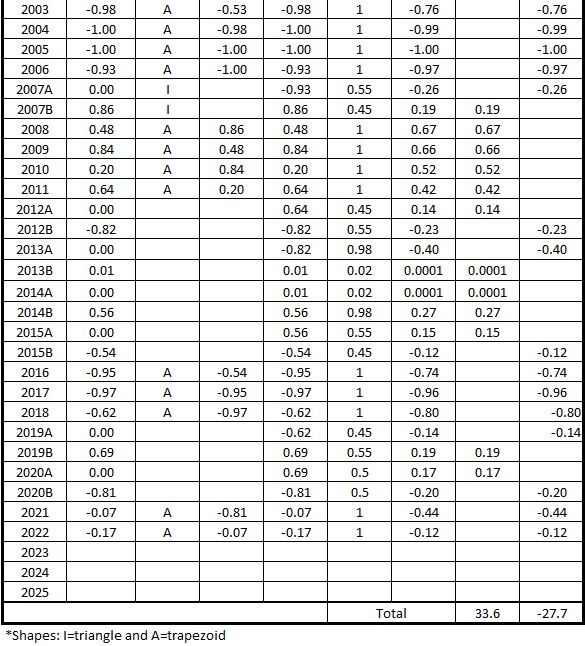
Much of the data plot in Figure 2 is defined by trapezoids.  There are also some triangles.  The dimensions for each shape are shown in Table 1, along with the calculated areas.

Table 1. U.S. Federal Deficits and Inflation  – Fiscal Years 1914-2022
(Area Under the Curve – Correlation, 3-Year Rolling Average)

Correlation of Inflation (Lagged 6 Months) with Deficit Spending

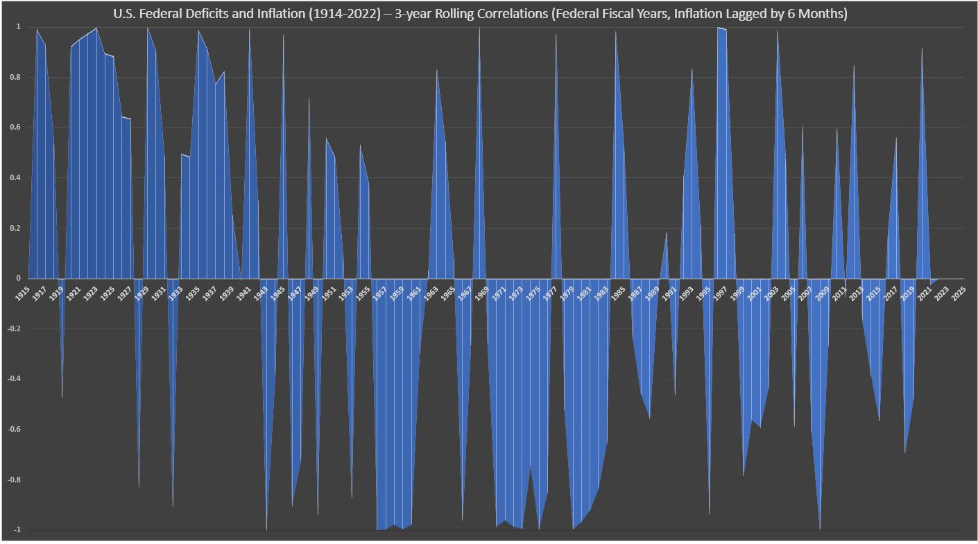
Figure 3 shows the 3-year rolling average of correlation when inflation is measured six months after the fiscal year deficit spending (compare to Figure 2 in Part 5¹).

Figure 3.  U.S. Federal Deficits and Inflation (Lagged 6 Months)
Fiscal Years 1914-2022
(Correlation, 3-Year Rolling Average)

Click here for larger image in a new window.  Exit new window (back arrow) to return to this page.

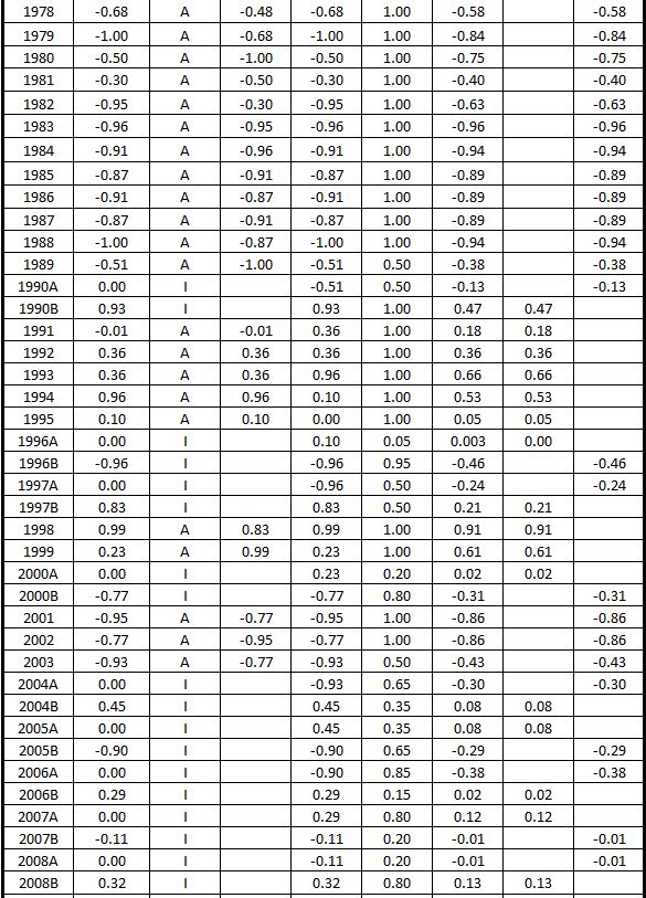
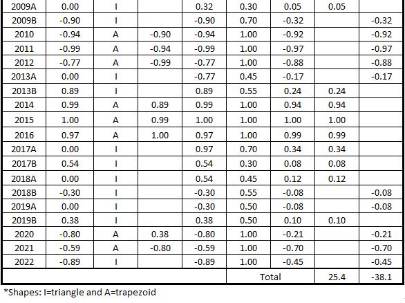
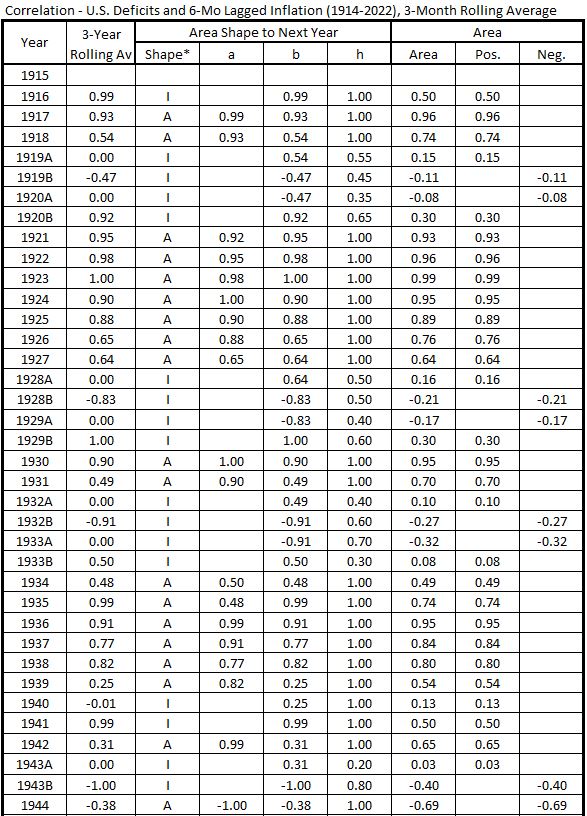
The dimensions for each shape in Figure 3 (above) are shown in Table 2, along with the calculated areas.

Table 2. U.S. Federal Deficits and Inflation (Lagged 6 Months)
Fiscal Years 1914-2022
(Area Under the Curve – Correlation, 3-Year Rolling Average)

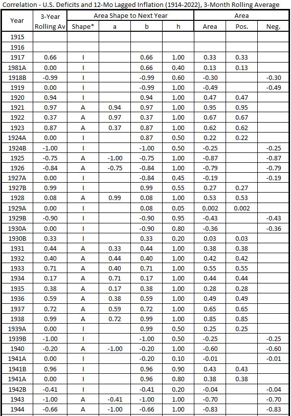
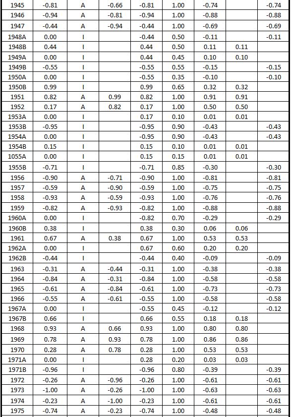
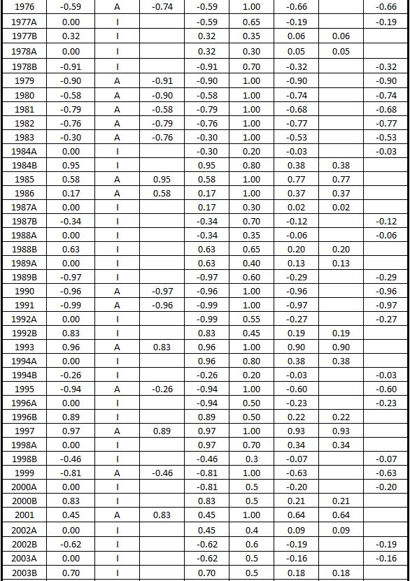
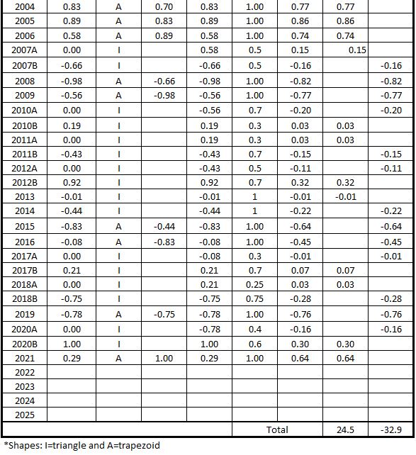
Correlation of Inflation (Lagged 12 Months) with Deficit Spending

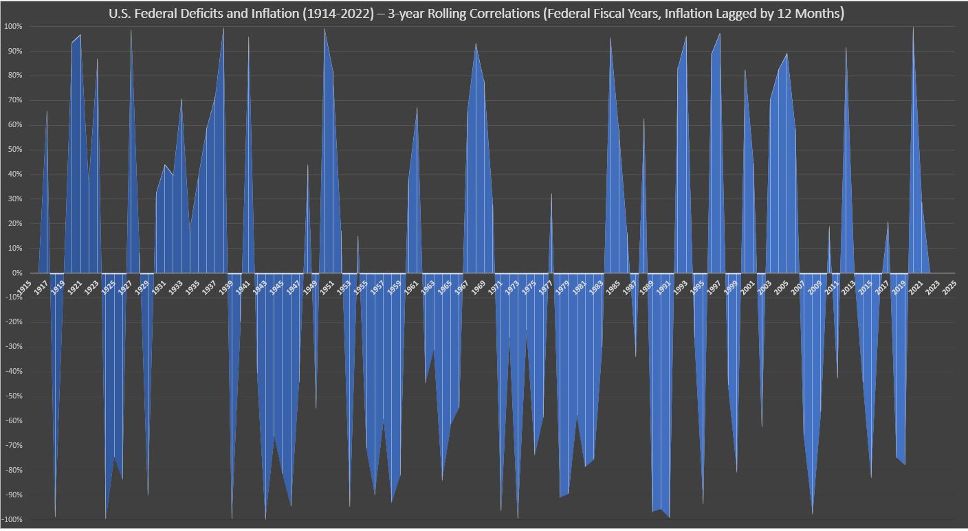
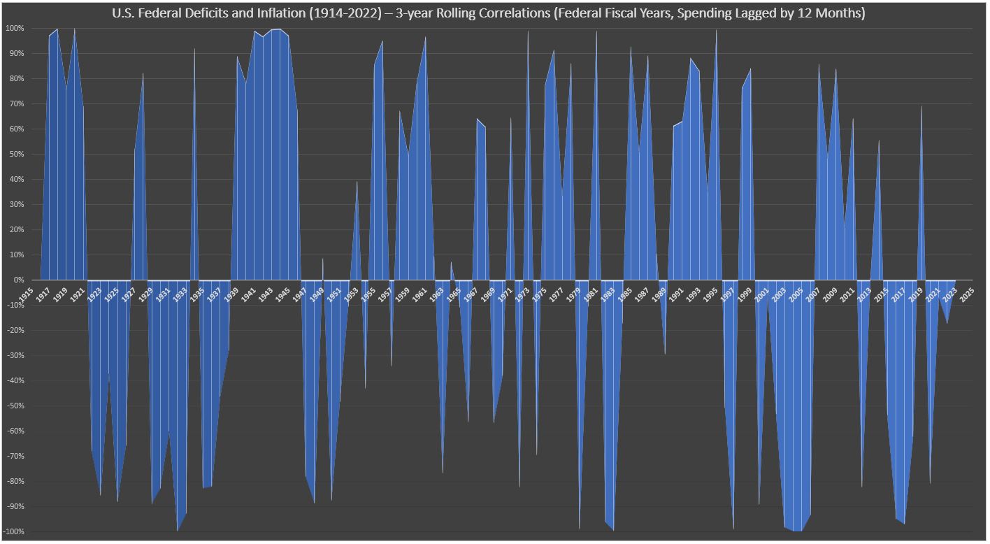
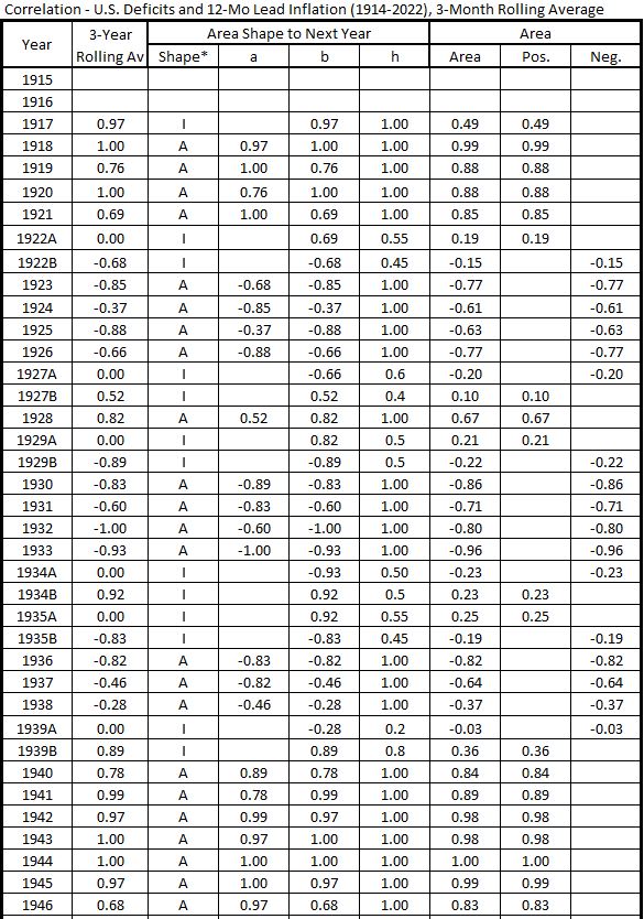
Figure 4 shows the 3-year rolling average of correlation when inflation is measured twelve months after the fiscal year deficit spending (compare to Figure 3 in Part 5¹).

Figure 4.  U.S. Federal Deficits and Inflation (Lagged 12 Months)
Fiscal Years 1914-2022
(Correlation, 3-Year Rolling Average)

Click here for larger image in a new window.  Exit new window (back arrow) to return to this page.

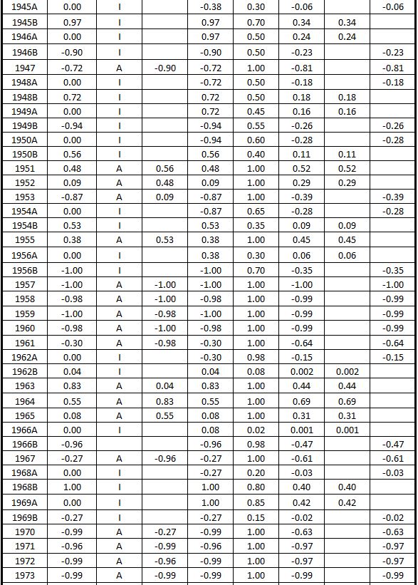
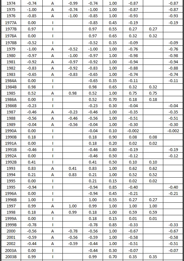
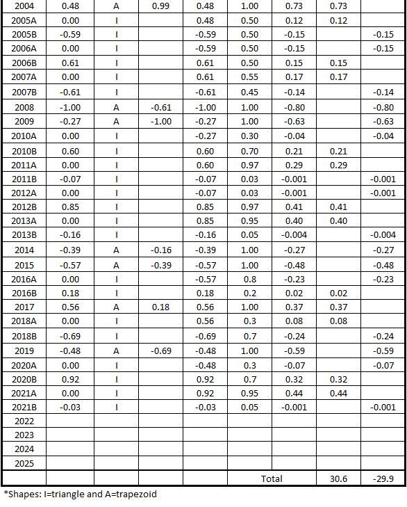
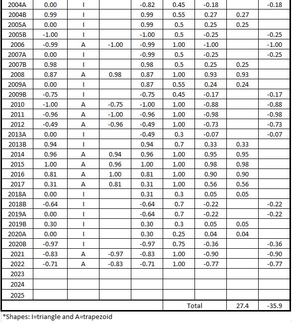
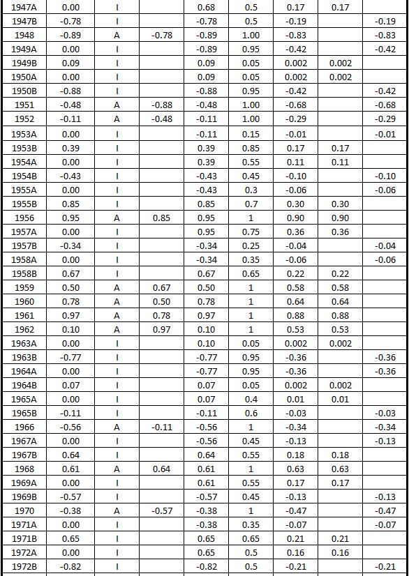
The dimensions for each shape in Figure 4 (above) are shown in Table 3, along with the calculated areas.

Table 3. U.S. Federal Deficits and Inflation (Lagged 12 Months)
Fiscal Years 1914-2022
(Area Under the Curve – Correlation, 3-Year Rolling Average)

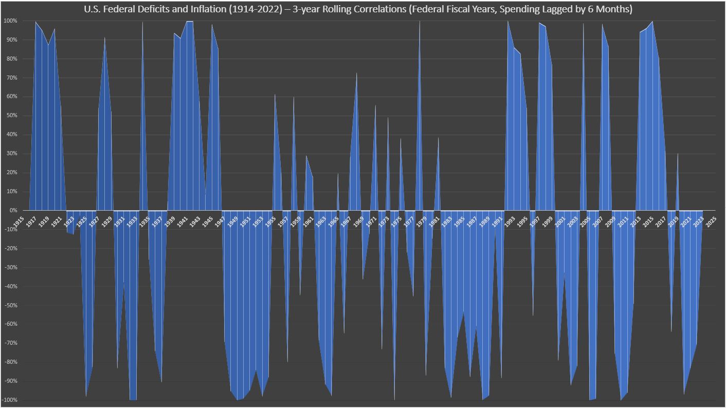
Correlation of Inflation (Leads by 6 Months) with Deficit Spending

Figure 5 shows the 3-year rolling average of correlation when inflation is measured six months before the fiscal year deficit spending (compare to Figure 4 in Part 5¹).

Figure 5.  U.S. Federal Deficits and Inflation (Leads 6 Months)
Fiscal Years 1914-2022
(Correlation, 3-Year Rolling Average)

Click here for larger image in a new window.  Exit new window (back arrow) to return to this page.

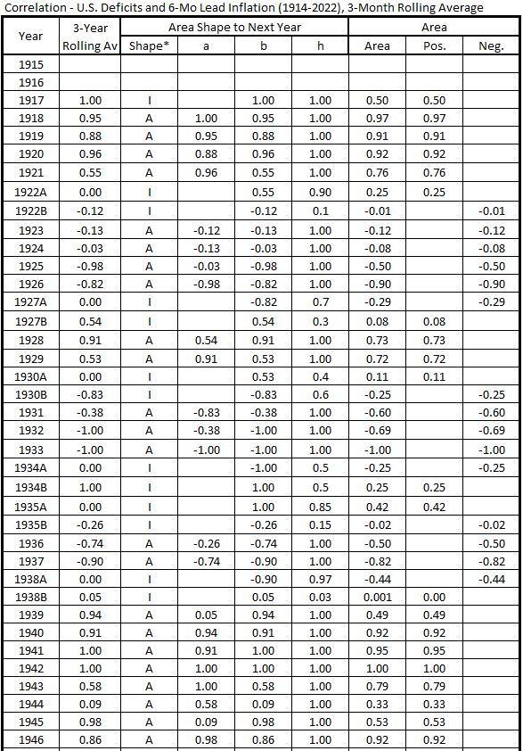
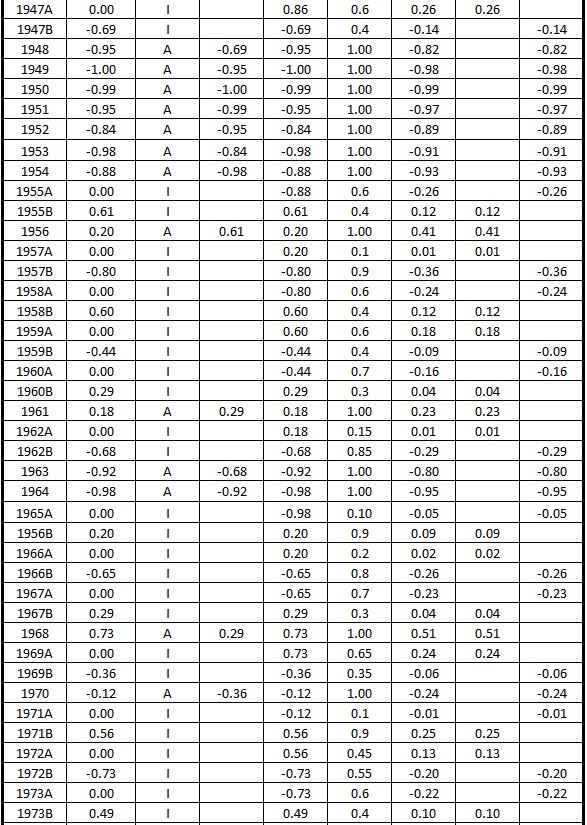
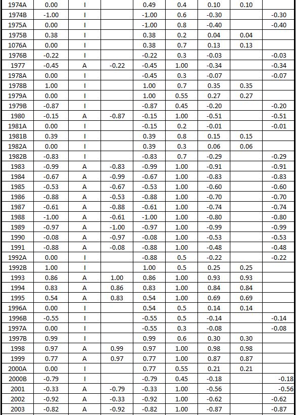
The dimensions for each shape in Figure 5 (above) are shown in Table 4, along with the calculated areas.

Table 4. U.S. Federal Deficits and Inflation (Leads 6 Months)
Fiscal Years 1914-2022
(Area Under the Curve – Correlation, 3 Year Rolling Average)

Correlation of Inflation (Leads by 12 Months) with Deficit Spending

Figure 6 shows the 3-year rolling average of correlation when inflation is measured twelve months before the fiscal year deficit spending (compare to Figure 5 in Part 5¹).

Figure 6.  U.S. Federal Deficits and Inflation (Leads 12 Months)
Fiscal Years 1914-2022
(Correlation, 3 Year Rolling Average)

Click here for larger image in a new window.  Exit new window (back arrow) to return to this page.

The dimensions for each shape in Figure 6 (above) are shown in Table 5, along with the calculated areas.

Table 5. U.S. Federal Deficits and Inflation (Leads 12 Months)
Fiscal Years 1914-2022
(Area Under the Curve – Correlation, 3 Year Rolling Average)

Analysis

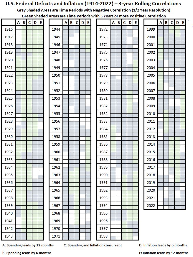
In Table 6, the gross quantitative features of the the correlations shown in the data are displayed.  The areas in gray are the years (or half-years in some cases) where the correlations are negative.  This shows there is no positive association of federal government deficit spending with inflation during those time periods.  The clear areas are for time periods less than three years in duration where positive correlation between deficit spending and inflation is found.  Because the data covers 3-year moving averages (rolling averages), this association is not considered as strong a relationship as the time periods colored green (three years and longer periods of positive association).

As a first pass evaluation of this data, the interpretation is that the positive correlations represent the maximum level of cause and effect that can exist between deficit spending and inflation during the green time periods.  It is also important to remember that the negative correlation periods indicate that there are times when there can be no direct cause and effect relationships between the two variables.  Table 7 summarizes these negative correlation periods.

Table 6. U.S. Federal Deficits and Inflation Correlation Patterns
3-Year Rolling Average 1916-2022 – Leads and Lags

Using the data in Table 6, the following table shows all the years when all correlations are negative.

Table 7.  U.S. Federal Deficits and Inflation, 3-Month Rolling Average 1916-2022
Time Periods With No Positive Correlation Possible

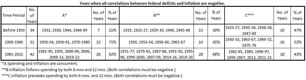
This data indicates there are many years when no positive correlations are possible over the sample period of 107 years.

The data summarized in Table 8 for significant positive correlations is derived from the tables in the Appendix.

Table 8.  U.S. Federal Deficits and Inflation, 3-Month Rolling Average 1916-2022
Number of Time Periods With Significant Positive Correlations

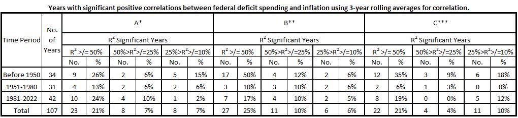
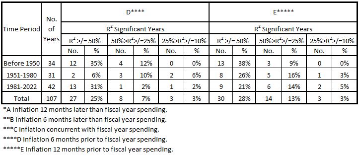
Less than half the years in the 107-year time period have significant positive correlations.  The highest percentage of years with significant positive correlations are seen for B (inflation following the fiscal year spending by six months) and for E (inflation preceding the fiscal year spending by twelve months).  I caution not to place any importance to this observation because all the other results are too close these two.

Conclusion

We believe we have gotten all the useful information we can from the data we have been organizing and interpreting.  Are we satisfied with the results?  The shortest answer is the best: No.

These results leave much to be desired.  We have not made a careful examination of how the use of 3-year rolling averages may have biased the results.  We used the smoothing technique because the year-by-year data was so noisy.  However, there may be useful information in that noise and it is worth the effort to dig into that possibility.

We also will investigate the effects of smoothing the data for each of the two variables before calculating correlations.  Our thoughts about that have raised the possibility that data-smoothing approach might produce different results.

The results obtained so far in this project are not without some value.  It is very evident that the association (correlation) of deficit spending with inflation within the time span +/- 1 year around the spending fluctuates wildly over the 108 years of data examined.  However, we think that applying more and different data organization processes can provide a clearer picture of how and when fluctuations occur.

Appendix

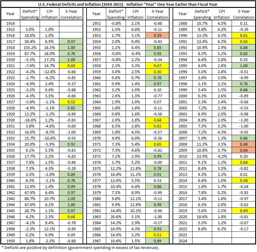
The following tables, A1 through A5, are Tables 1-5 posted previously,³ with added notations as follows:

• Green for 3-Year Correlation values ≥0.707.
• Yellow for 0.707> 3-Year Correlation values ≥0.5.
• Red for 0.5> 3-Year Correlation values ≥0.316.

The correlation coefficients correspond to R² values of 50%, 25%, and 10%.  These are selected to define three significant levels for association of the two variables, deficit spending and inflation.

Table A1.  U.S. Federal Deficits and Inflation – Fiscal Years 1914-2022

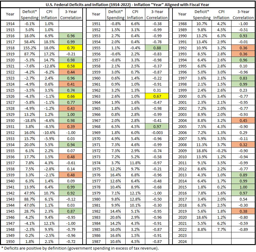
Table A2.  U.S. Federal Deficits and Inflation – Fiscal Years 1914-2022
(Deficits Lead Inflation by 6 Months)

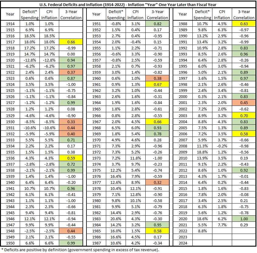
Table A3.  U.S. Federal Deficits and Inflation – Fiscal Years 1914-2022
(Deficits Lead Inflation by 12 Months)

Table A4.  U.S. Federal Deficits and Inflation – Fiscal Years 1914-2022
(Deficits Trail Inflation by 6 Months)

 

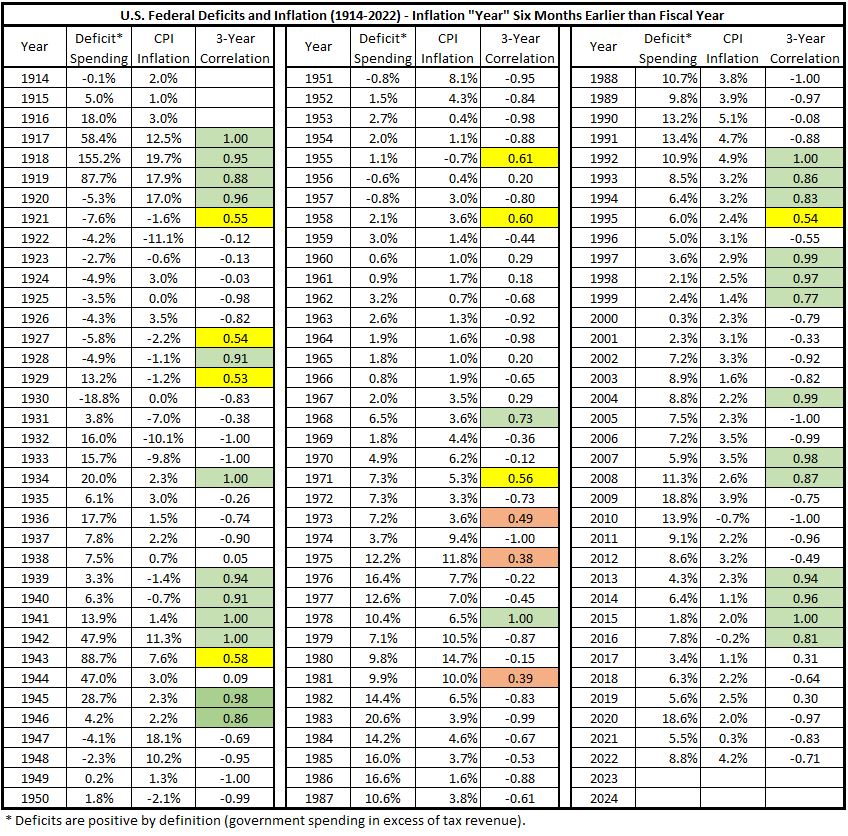
Table A5.  U.S. Federal Deficits and Inflation – Fiscal Years 1914-2022
(Deficits Trail Inflation by 12 Months)

 

Footnotes

1.  Lounsbury, John, “Government Spending and Inflation. Part 4”, EconCurrents, March 5, 2023. https://econcurrents.com/2023/03/05/government-spending-and-inflation-part-4/.

2. Lounsbury, John, “Measuring Area Under a Curve in Excel”, EconCurrents, March 19, 2023.  https://econcurrents.com/2023/03/19/measuring-area-under-a-curve-in-excel/.

3. Lounsbury, John, “Government Spending and Inflation. Part 5”, EconCurrents, March 12, 2023. https://econcurrents.com/2023/03/12/government-spending-and-inflation-part-5/.