Government Spending and Inflation. Part 5

We have previously¹ used the CPI data available since 1913 to create annualized inflation data aligned with the federal fiscal years from 1914 to 2022.  In this post, we use the timeline-matched data to examine leads or lags that may exist between the two variables – government spending and inflation.

Credit:  Photo by Ann H from Pexels

Introduction

The hypothesis that federal government deficit spending is a cause of inflation in the general economy has been in vogue for some time.  For the Nobel Laureate economist Milton Friedman, it was a cornerstone consequence of his monetary theory.²

The effect of increased deficit spending on inflation may not be immediate (coincident).  If there is a delay in the assimilation of the additional money in the general economy, it would show up in an increased correlation between the two variables with a lag between government spending and the increase in inflation.  In this report, we will look for such a lag.

We will also examine how correlation varies if the lead/lag relationship is reversed.  If positive correlation increases when increased government spending occurs after increased inflation in the economy, the hypothesis of deficit spending would need reconsideration.

Data

The data used for the calculations here comes from Table 1, Table 2, and Table 3 in Part 4 of this series.¹

Deficits Coincident with Inflation

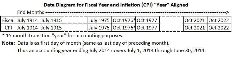
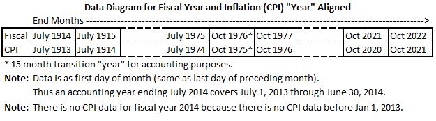
The inflation data comes from the July column in Table 2 for 1914-1975 and the October column for 1977-2022.  There is an extra quarter after the 1976 fiscal year (July 1, 1975, to June 30, 1976) in the transition to fiscal year 1977 (starting October 1, 1976).  This transition quarter has been added to the numbers for fiscal year 1976.³  To align with the fiscal data adjustment, the inflation data has been calculated (Using Table 1 in Part 4) from the change in the CPI values for the 15 months between July 1, 1975, and October 1, 1976 (57.9-54.2 = 3.7 or 6.8%).

The government deficit spending for each fiscal year is taken from Table 3 in Part 4.

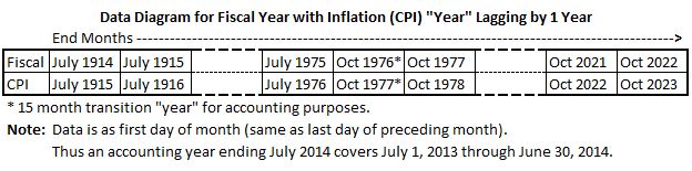
The discussion above is conveniently summarized with a data diagram:

Following the data diagram above, the data has been extracted from then Tables in Part 4.

Table 1.  U.S. Federal Deficits and Inflation  – Fiscal Years 1914-2022

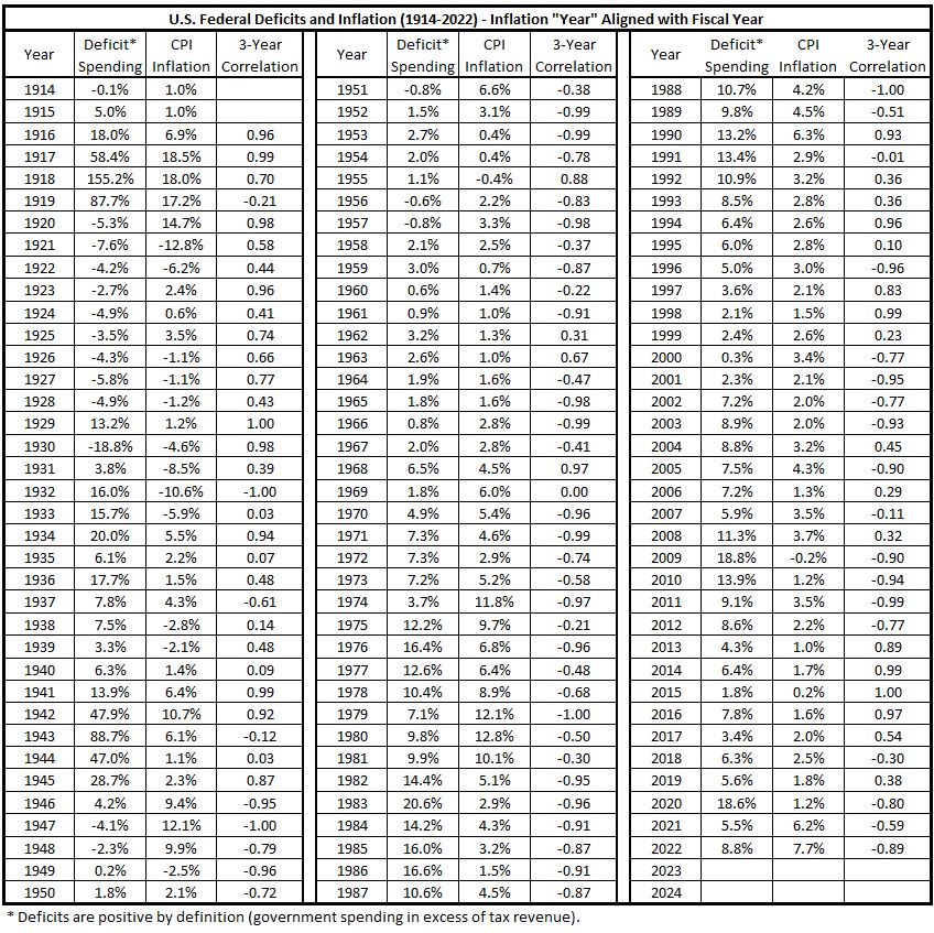
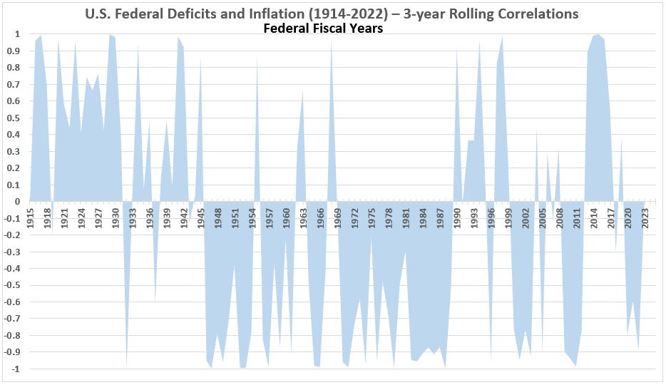
Figure 1.  U.S. Federal Deficits and Inflation  – Fiscal Years 1914-2022
(Correlation, 3 Month Rolling Average)

 

Deficits Leading Inflation

Deficits vs. Inflation Six Months Later

The data diagram is summarized as follows:

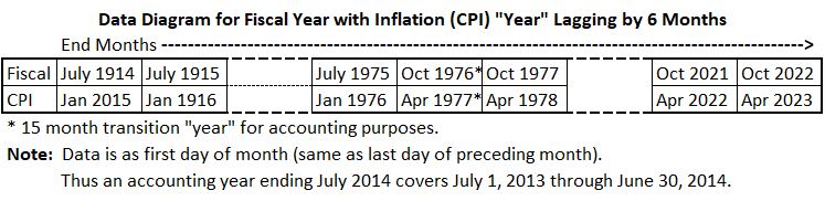
For aligning inflation to the transition year in Table 2, the 15 month window for inflation lagging 6-months after government spending is the change in CPI from Jan. 1, 1976, and Apr. 1, 1977 (60.0-55.6 = 4.4 or 7.9%).

Table 2.  U.S. Federal Deficits and Inflation  – Fiscal Years 1914-2022
(Deficits Lead Inflation by 6 Months)

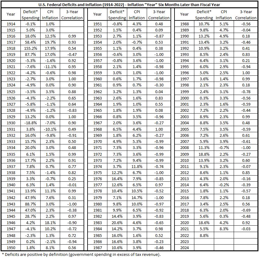
At the time this is written (March 13, 2023), the CPI data necessary to align with the 6-month delay for fiscal year 2022 is not yet available.

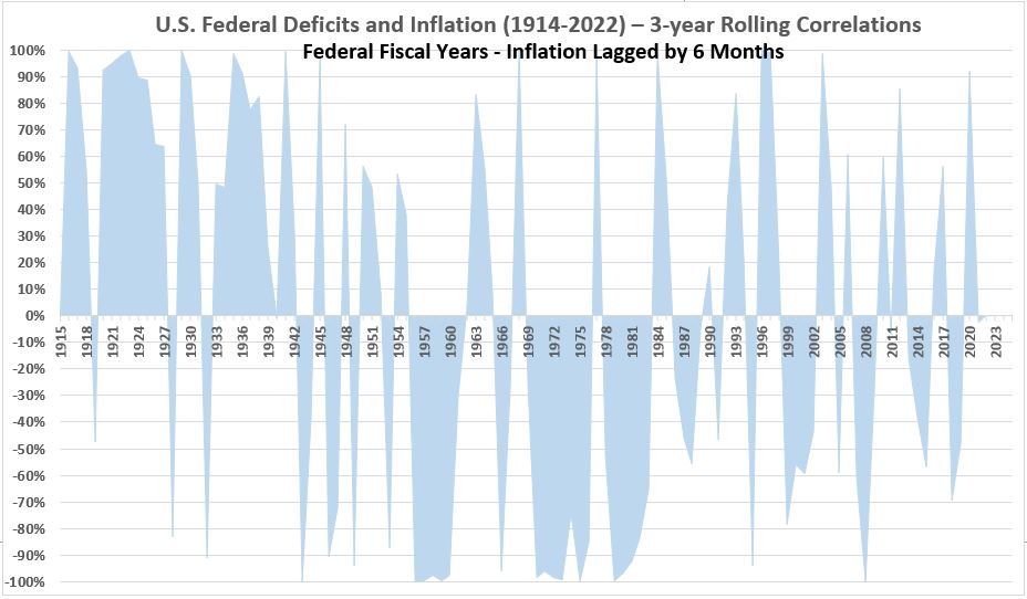
Figure 2.  U.S. Federal Deficits and Inflation  – Fiscal Years 1914-2022
3-Month Correlation Rolling Average
(Deficits Lead Inflation by 6 Months)

Deficits vs. Inflation One Year Later

The data diagram is summarized as follows:

The 15 month window for the transition period of inflation lagged 12 months is the change in CPI from July 1, 1976, and Oct. 1, 1977 (61.6-57.1 = 4.5 or 7.9%)

Table 3.  U.S. Federal Deficits and Inflation  – Fiscal Years 1914-2022
(Deficits Lead Inflation by 12 Months)

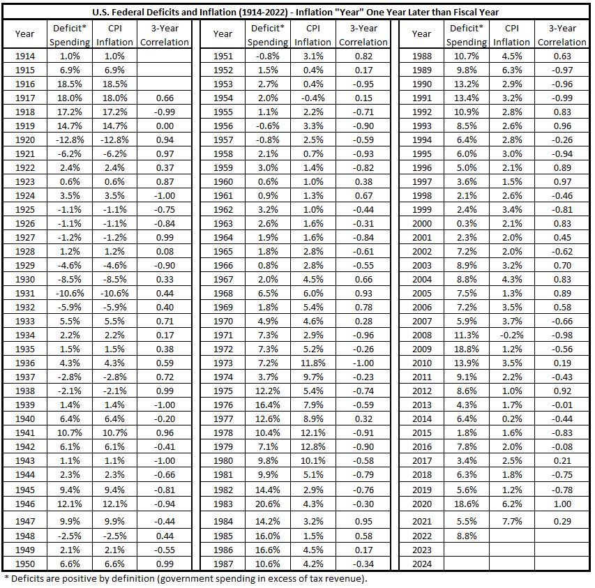
At the time this is written (March 13, 2023), the CPI data necessary to align with the 1-year delay for fiscal year 2022 is not yet available.

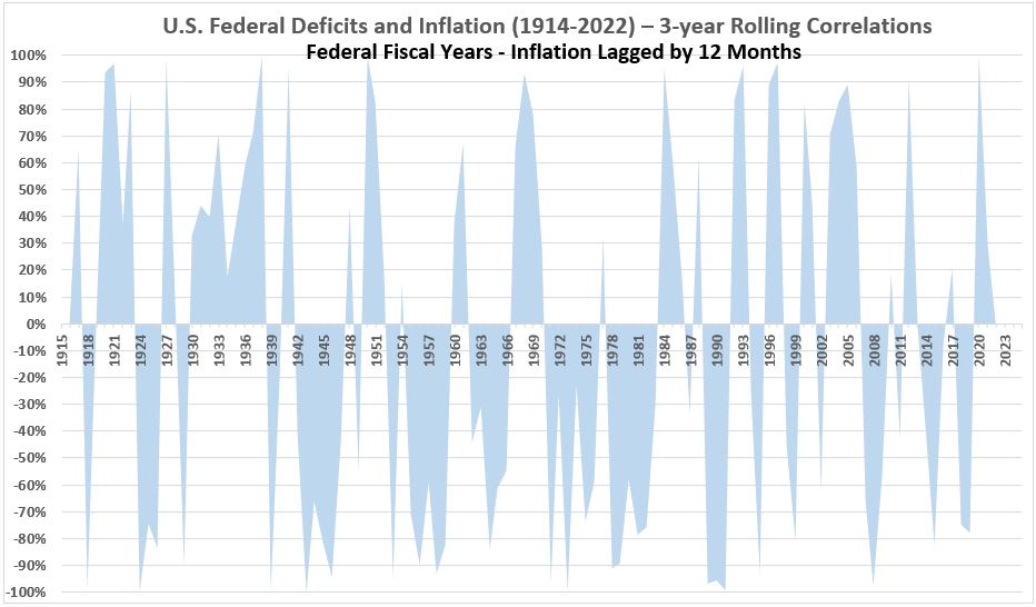
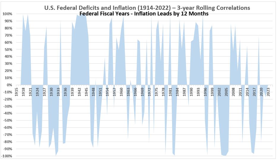
Figure 3.  U.S. Federal Deficits and Inflation  – Fiscal Years 1914-2022
3-Month Correlation Rolling Average
(Deficits Lead Inflation by 12 Months)

 

Inflation Leading Deficits

Deficits vs. Inflation Six Months Earlier

The data diagram is summarized as follows:

When inflation leads spending by 6 months, the 15 month transition period for inflation is the change in CPI from Jan. 1, 1975 to Apr. 1, 1976 (56.1-52.1 = 4.0 or 7.7%).

Table 4.  U.S. Federal Deficits and Inflation  – Fiscal Years 1914-2022
(Deficits Trail Inflation by 6 Months)

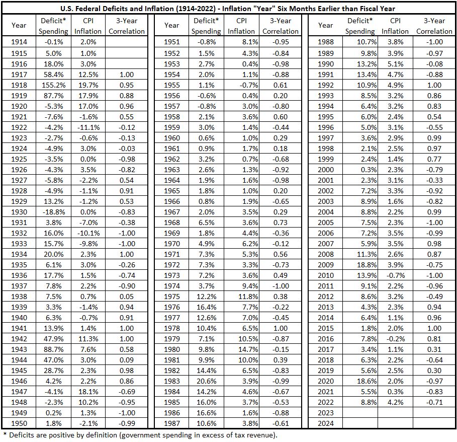
Figure 4.  U.S. Federal Deficits and Inflation  – Fiscal Years 1914-2022
3-Month Correlation Rolling Average
(Deficits Trail Inflation by 6 Months)

 

Deficits vs. Inflation One Year Earlier

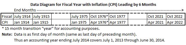
The data diagram is summarized as follows:

When inflation leads spending by 12 months, the 15 month transition period for inflation is the change in CPI from July 1, 1974 to Oct. 1, 1975 (54.9-49.4 = 5.5 0r 11.1%).

Table 5.  U.S. Federal Deficits and Inflation  – Fiscal Years 1914-2022
(Deficits Trail Inflation by 12 Months)

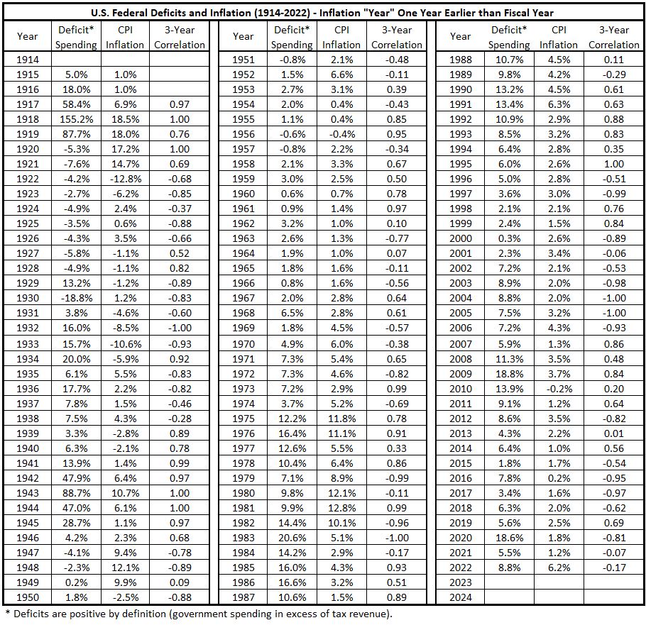
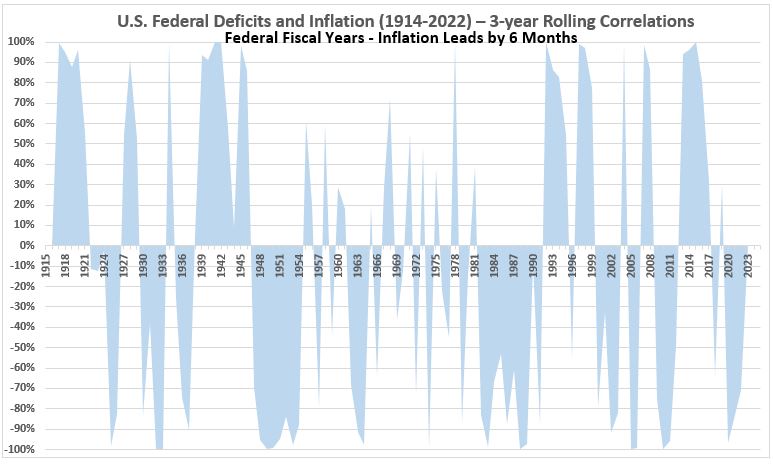
Figure 5.  U.S. Federal Deficits and Inflation  – Fiscal Years 1914-2022
3-Month Correlation Rolling Average
(Deficits Trail Inflation by 12 Months)

Analysis

There is limited analysis that seems appropriate at this stage of development.  It is tempting to say that Figure 1 shows the most negative correlation pattern of the five graphs above.  Also it seems that Figure 5 may show the  most positive correlation pattern, while the other three graphs are more evenly balanced between the amounts of positive and negative correlation.  These observations are qualitative and preliminary.

Further consideration of what the five graphs produced suggests we should wait for more quantitative analysis which will be attempted in the coming week.

Another important feature of the graphs is that the more careful timeline alignment of the data has not changed the large number of wild swings in correlation over the 109 year period 1914-2022, compared to our earlier work with less precise data.^4,5  This seemingly infers that the amount of association between deficit spending and inflation varies widely over relatively short periods of time.

Conclusion

We have not yet arrived at any quantitative analysis of the data.  But the qualitative observations indicate that the association between deficit spending and inflation may be far from a simple cause and effect relationship.  And, whatever the relationship may turn out to be, it will certainly be strongly time-variant.

Appendix

Interpretation of Correlation Coefficients

The association between two variables in an observation or an experiment is measured by calculating the correlation coefficient, R.  In the instance of this examination of the relationship between government spending and inflation, we are dealing with observations.

With observations, there is not necessarily a defined mathematical relationship between the variables.  However, there has been an assumed linear relationship between money and inflation.

Milton Friedman famously declared:²

“Inflation is created in Washington because only Washington can create money.”⁶

Because of the long-held belief that government spending is an important driver (according to Friedman, the important driver²) of inflation, the current investigation has been developed.

A traditional way of determining correlation between two variables is by means of regression analysis of a scatterplot graph.⁹

The data used in Figure 1 (above) for the two variables federal government deficit spending (X) and year-over-year inflation measured for the fiscal year (Y) are displayed in the graph below:

Figure 6.  Scatterplot for Inflation Dependent on Federal Government Deficit Spending (1914-2022)

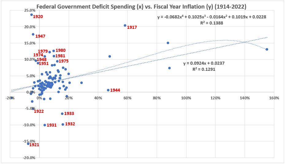
The linear regression is shown to represent the relationship expected for Friedman’s hypothesis.  The fourth power polynomial regression is presented to show that higher power polynomial fits to the data are not significantly better than the linear relationship.  A higher power polynomial is not considered an appropriate model, this is just an illustration.

Sixteen data points are date labelled.  These are the sixteen years that deviate from the linear regression by more than 5% year-over-year inflation.  The data for the remaining 93 years is plotted in Figure 7.  There is no reason for doing this at the present time except to show how big was the influence of the outlying data points.

Figure 7.  Scatterplot for Inflation Dependent on Federal Government Deficit Spending (1914-2022)
Outliers Omitted

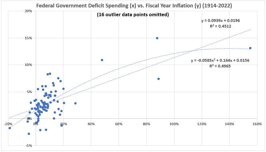
Figure 7 shows how omitting outliers can drastically change the correlation results in this case.  The functional form of the model is little changed (ie, the values of m and b in Figure7 are little changed from those in Figure 6X) .

y = mx +b

There is no model proposed that has the quadratic form shown in the graph.  That is displayed for comparison purposes only.  The correlation result is slightly better for th quadratic fit, but the difference is too small to call into question the linear form of the model.

The 16 outlier data points omitted were from four groups of closely spaced (many were consecutive) years.  The significance of these observations is that it encourages the idea of looking at the relationship between inflation and deficit spending in those groups of years uninterupted by outliers.  There are four such groups, consisting of 9 years (1923-1930), 11 years (1934-1943), 23 years (1952-1973), and 41 years (1982-2022).

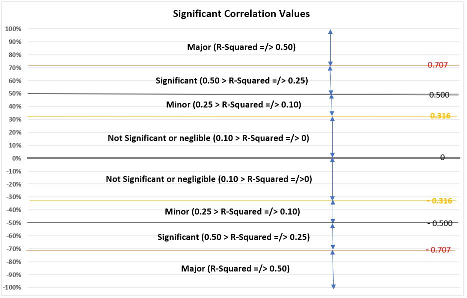
Figure 8 defines what we have defined to be important correlation thresholds to consider.

Figure 8.  Important Values of Correlation Coeficients (R)

 

Footnotes

1.  Lounsbury, John, “Government Spending and Inflation. Part 4”, EconCurrents, March 5, 2023. https://econcurrents.com/2023/03/05/government-spending-and-inflation-part-4/

2.  Friedman, Milton, “Only Government Creates Inflation”, YouTube, https://youtu.be/F94jGTWNWsA.

3.  The Department of the Treasury, Document No. 3269, COMBINED STATEMENT OF RECEIPTS, EXPENDITURES AND BALANCES OF THE UNITED STATES GOVERNMENT FOR THE FISCAL YEAR ENDED JUNE 30, 1976 AND THE TRANSITION QUARTER ENDED SEPTEMBER 30, 1976, Stock Number 048 — 008 — 00011 — 9, Catalog Number T63. 113;975, https://www.govinfo.gov/content/pkg/GOVPUB-T63-aa06fae6dd8e856a4126668c7662a25d/pdf/GOVPUB-T63-aa06fae6dd8e856a4126668c7662a25d.pdf.

4. Lounsbury, John, “Government Spending and Inflation. Part 2”, EconCurrents, February 19, 2023. https://econcurrents.com/2023/02/19/government-spending-and-inflation-part-2/

5.  Lounsbury, John, “Government Spending and Inflation. Part 3”, EconCurrents, February 26, 2023.  https://econcurrents.com/2023/02/26/government-spending-and-inflation-part-3/

6.  Of course, this statement is completely incorrect.  Friedman ignored the private sector creation of credit, because he (as did many other economists) did not include money in economic theory.  Instead, money was dismissed as an unimportant element of economic theory under the now discredited loanable funds theory model of banking.^7,8

7.  Werner, Richard A., “Can banks individually create money out of nothing? — The theories and the empirical evidence”, International Review of Financial Analysis, Volume 36, December 2014, Pages 1-19.

8.  Jakab, Zoltan and Kumhof, Michael, “Banks are not intermediaries of loanable funds — facts, theory and evidence”, Staff Working Paper No. 761, Bank of England, October 26, 2018, Updated June 2019.  https://www.bankofengland.co.uk/-/media/boe/files/working-paper/2018/banks-are-not-intermediaries-of-loanable-funds-facts-theory-and-evidence.pdf

9.  Adler, Henry L. and Roessler, Edward B., Introduction to Probabilty and Statistics, Fifth Edition, W.H. Freeman and Company, San Francisco, 1972.  Chapter 12, pp 195-226.